Mukul Kumar Gupta* | Paawan Sharma | Nitish Sinha | Adesh Kumar | Varnita Verma
© 2021 IIETA. This article is published by IIETA and is licensed under the CC BY 4.0 license (http://creativecommons.org/licenses/by/4.0/).
OPEN ACCESS
In this article, we study the machine learning based regression analysis of triple link distributed pendulum (TLDP) under free condition for estimation of natural frequency of each link of the pendulum. The modeling of the triple link pendulum based on Euler-Lagrange technique which is also proposed by Gupta et al. It is observed that the bottom link of the pendulum has higher frequency corresponding to the top and middle pendulum of the link. However, the frequency of the pendulum link increases from top to bottom link with decreases the deviation angle of TLDP. This result is also confirming with different algorithms of the machine learning technique. Real time model has also been developed to verify the frequency analysis of the system. Decision tree regression (DTR) technique estimate better frequency for the top and middle pendulum link. However, random forest regression (RFR) technique is better estimation of frequency the bottom link of the pendulum.
decision tree, Euler Lagrange, triple link pendulum, time series analysis
An enormous and broad study relating to the pendulum, including a historical review, is presented by Baker and Blackburn [1]. The multilink pendulum type system represents behaviors such as frequency transformation, time series behavior, non-local dynamic behavior, visual recurrence and resonance behavior [2-4]. The pendulum has a wide variety of application in the control and robotics related area since its inception. Single and double pendulums theoretical and experimental investigations [5] are present in a good number. The planar triple physical pendulum system dynamic analysis with no external forces was investigated numerically by Gupta et al. [6], where different cases for both lumped and distributed case have been considered. Recurrence plot (visual representation of system properties) analysis for triple pendulum system has been discussed by Gupta et al. [3] and asserts that chaotic behavior increases with degree of freedom but for small angle multilink pendulum shows periodic or quasiperiodic motion.
The triple link pendulum has many applications invalidating nonlinear control technique, dynamics of robot manipulator, biomechanics, cranes, automatic aircraft landing system and robogymnast and human upper limb motion [7, 8] also. Because of all these applications and rich nonlinear behavior triple link pendulum has gained lot of attraction among research community.
The simulation of system model generates corresponding time series data. Time series analysis is the study of data collected successively in time. This consists of linear/nonlinear discrete-time model representations. Time series analysis is very important as many prediction problems involve a time dependent component. The time series analysis for double pendulum system has been studied by Yao [9] and Gupta et al. [10] and also the chaotic behavior based on mass and length has been discussed. Various signal-processing tools are available to evaluate the model parameters. The study related to patterns inherent in time-series have been extensively analyzed in the area of nuclear reactor [11], solar PV grid [12], Mars environment [13], underwater glider [14].
The outcome of time series analysis is highly useful in generating data which can be used as input to various machine learning modelling process [15]. The area of machine learning is becoming quite popular in solving various problems in multiple domains of control system [16-18]. In order to perform the desired system trajectory various control techniques were implemented in literature [19-21]. Machine learning is advanced mathematical method of analyzing signals and used to develop methods for detecting patterns present in the signal, and also to detect similar patterns in different dataset [18]. The main advantage of machine learning is the ease with which it can be applied to big sized data. The type of learning method can be divided into supervised, unsupervised and reinforcement learning. Supervised learning makes use of input-output relationship for a given system, while unsupervised focuses on the inputs alone to generate a data knowledge map grouping similar data together. On the other hand, reinforcement learning is based on reward-penalty system depending on the importance of outcome. Amongst these methods, supervised learning is most commonly used since it considers output data as well while observing input-output relationship for given system data. The type of prediction can be either a class prediction (classification) or estimating a parameter value (regression). The regression methods include various techniques such as simple linear regression (SLR), multiple linear regression (MLR), support vector regression (SVR), polynomial regression, decision tree regression (DTR) and random forest regression (RFR).
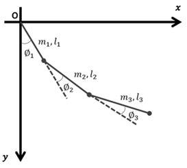
The triple link pendulum system as a distributed mass and length under free conditions (no applied torque at each joint) is shown in Figure 1. The system has three masses m1, m2 and m3 and three length l1, l2, and l3 respectively. Each mass is uniformly distributed throughout the link length and links are rigid in nature. No frictional coupling is available between the links. The triple link distributed system is assumed to be in fourth quadrant. The angles from each joint are represented by ∅_1, ∅_(2,) and ∅_3 respectively.
Figure 1. Triple Link Pendulum as a distributed mass and length
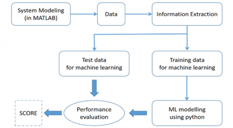
The dynamic modelling of triple link pendulum system has been obtained using Euler -Lagarange technique and given by Gupta et al. [6]. Figure 2 represents the complete analysis flow in the present study.
Figure 2. Process flow for the analysis of TLDP
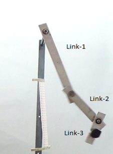
Figure 3 shows the real time triple link pendulum model developed in the laboratory.
This paper focuses on performance of regression techniques namely MLR, DTR and RFR for estimation of time period associated with the angular velocity of arms of triple pendula. Figure 4 shows the learning process flow.
Figure 3. Developed triple link pendulum model
Figure 4. Machine learning modeling process
This section consists of results for Time series and FFT analysis, and machine learning modelling followed by its discussion.
4.1 Time Series and FFT Analysis
Figures 5-10 show time series and FFT plots for two different data points of the pendula links ${{l}_{1}}$, ${{l}_{2}}$and ${{l}_{3}}$ respectively. The time series and Fast Fourier Transform (FFT) analysis have been obtained for different initial conditions. For Figure 5, Figure 7 & Figure 9, the initial values for the angles are $\left( \frac{\pi }{10},0,\frac{\pi }{6},0,\frac{\pi }{10},0 \right)$ radian, length ${{l}_{1}},{{l}_{2}},{{l}_{3}}$ are taken as 6,6,14 units respectively and corresponding mass ${{m}_{1}},{{m}_{2}},{{m}_{3}}$ are taken as 10, 8 and 5 units respectively. For Figure 6, Figure 8 & Figure 10, the initial values for the angle are$\left( \frac{\pi }{4},0,\frac{\pi }{4},0,\frac{\pi }{4},0 \right)$radian; length ${{l}_{1}},{{l}_{2}},{{l}_{3}}$ and corresponding mass ${{m}_{1}},{{m}_{2}},{{m}_{3}}$ are taken as unity.
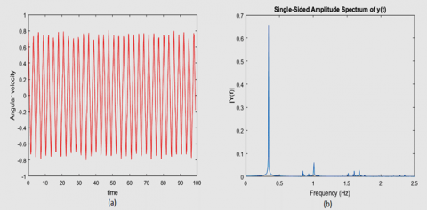
Figure 5. Time-series plot and corresponding frequency spectrum for different parameter values of pendulum for Link ${{l}_{1}}$ [${{\varphi }_{1}},{{\varphi }_{2}},{{\varphi }_{3}}$)=$\left( \frac{\pi }{10},0,\frac{\pi }{6},0,\frac{\pi }{10},0 \right)$, (${{l}_{1}},{{l}_{2}},{{l}_{3}}$ = 6,6,14), (${{m}_{1}},{{m}_{2}},{{m}_{3}}$= 10,8,5)]
Figure 6. Time-series plot and corresponding frequency spectrum for different parameter values of pendulum for Link ${{l}_{1}}$ [ (${{\varphi }_{1}},{{\varphi }_{2}},{{\varphi }_{3}}$)=$\left( \frac{\pi }{10},0,\frac{\pi }{6},0,\frac{\pi }{10},0 \right)$, (${{l}_{1}},{{l}_{2}},{{l}_{3}}$ = 1,1,1), (${{m}_{1}},{{m}_{2}},{{m}_{3}}$= 1,1,1)]
Figure 7. Time-series plot and corresponding frequency spectrum for different parameter values of pendulum for Link ${{l}_{2}}$[ (${{\varphi }_{1}},{{\varphi }_{2}},{{\varphi }_{3}}$)=$\left( \frac{\pi }{10},0,\frac{\pi }{6},0,\frac{\pi }{10},0 \right)$, (${{l}_{1}},{{l}_{2}},{{l}_{3}}$ = 6,6,14), (${{m}_{1}},{{m}_{2}},{{m}_{3}}$= 10,8,5)]
As shown in Figure 5, from FFT analysis it is clear that if more than one peak is available then chances of periodicity will be less. From the literature, it is clear that periodic doubling is a sign of chaos or the system leads to chaos. It is clear from time series analysis that system is aperiodic. In this case, it is more of quasi periodic in nature. The following results are for the first angular velocity.
From Figure 6, it is clear that one dominant frequency is present. This time series plot reflects periodic behavior and hence, only one peak is available in FFT. The value of the frequency is 0.3369 Hz. Similar behavior can be observed for different cases as shown in Figures 7-10.
Figure 8. Time-series plot and corresponding frequency spectrum for different parameter values of pendulum for Link ${{l}_{2}}$[ (${{\varphi }_{1}},{{\varphi }_{2}},{{\varphi }_{3}}$)=$\left( \frac{\pi }{4},0,\frac{\pi }{4},0,\frac{\pi }{4},0 \right)$, (${{l}_{1}},{{l}_{2}},{{l}_{3}}$ = 1,1,1), (${{m}_{1}},{{m}_{2}},{{m}_{3}}$= 1,1,1)]
Figure 9. Time-series plot and corresponding frequency spectrum for different parameter values of pendulum for Link ${{l}_{3}}$[ (${{\varphi }_{1}},{{\varphi }_{2}},{{\varphi }_{3}}$)=$\left( \frac{\pi }{10},0,\frac{\pi }{6},0,\frac{\pi }{10},0 \right)$, (${{l}_{1}},{{l}_{2}},{{l}_{3}}$ = 6,6,14), (${{m}_{1}},{{m}_{2}},{{m}_{3}}$= 10,8,5)]
Figure 10. Time-series plot and corresponding frequency spectrum for different parameter values of pendulum for Link ${{l}_{3}}$[ (${{\varphi }_{1}},{{\varphi }_{2}},{{\varphi }_{3}}$)=$\left( \frac{\pi }{4},0,\frac{\pi }{4},0,\frac{\pi }{4},0 \right)$, (${{l}_{1}},{{l}_{2}},{{l}_{3}}$ = 1,1,1), (${{m}_{1}},{{m}_{2}},{{m}_{3}}$= 1,1,1)]
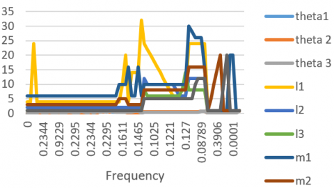
Table 1 also represent some of the data points for ${{l}_{1}}$ link, similarly other data points are calculated for ${{l}_{2}}$and ${{l}_{3}}$ link. Figure 11, 12 and 13 represents the data obtained with the system modeling and simulation in MATLAB for TLDP. This data consists of initial angle of individual links, lengths and mass of the links, and dominant frequency of oscillations. Total 68 different cases have been considered under different conditions. The frequency component having maximum magnitude in FFT analysis have been selected as the frequency of oscillation for various values of mass, length and angle of TLDP.
Table 1. System data for ${{l}_{1}}$ link
|
$\theta_{1}$ |
$\theta_{2}$ |
$\theta_{3}$ |
$l_{1}$ |
$l_{2}$ |
$l_{3}$ |
$m_{1}$ |
$m_{2}$ |
$m_{3}$ |
$F(\mathrm{~Hz})$ |
|
0 |
0 |
0 |
4 |
2 |
1 |
6 |
3 |
1 |
0 |
|
π/4 |
0 |
0 |
4 |
2 |
1 |
6 |
3 |
1 |
0.2393 |
|
0 |
π/4 |
0 |
4 |
2 |
1 |
6 |
3 |
1 |
0.2344 |
|
0 |
0 |
π/4 |
4 |
2 |
1 |
6 |
3 |
1 |
0.542 |
|
π/6 |
0 |
0 |
4 |
2 |
1 |
6 |
3 |
1 |
0.2344 |
|
0 |
π/6 |
0 |
4 |
2 |
1 |
6 |
3 |
1 |
0.2344 |
|
0 |
0 |
π/6 |
4 |
2 |
1 |
6 |
3 |
1 |
0.5469 |
|
π/10 |
0 |
0 |
4 |
2 |
1 |
6 |
3 |
1 |
0.2344 |
|
0 |
π/10 |
0 |
4 |
2 |
1 |
6 |
3 |
1 |
0.2344 |
|
0 |
0 |
π/10 |
4 |
2 |
1 |
6 |
3 |
1 |
0.5518 |
|
π/4 |
π/6 |
0 |
4 |
2 |
1 |
6 |
3 |
1 |
0.2246 |
|
π/4 |
π/10 |
0 |
4 |
2 |
1 |
6 |
3 |
1 |
0.2295 |
|
π/4 |
0 |
π/6 |
4 |
2 |
1 |
6 |
3 |
1 |
0.2344 |
|
π/4 |
0 |
π/10 |
4 |
2 |
1 |
6 |
3 |
1 |
0.2441 |
|
π/6 |
π/4 |
0 |
4 |
2 |
1 |
6 |
3 |
1 |
0.2295 |
|
π/6 |
π/10 |
0 |
4 |
2 |
1 |
6 |
3 |
1 |
0.2295 |
|
π/6 |
0 |
π/4 |
4 |
2 |
1 |
6 |
3 |
1 |
0.2344 |
|
π/6 |
0 |
π/10 |
4 |
2 |
1 |
6 |
3 |
1 |
0.2344 |
|
π/10 |
π/4 |
0 |
4 |
2 |
1 |
6 |
3 |
1 |
0.2295 |
|
π/10 |
0 |
π/4 |
4 |
2 |
1 |
6 |
3 |
1 |
0.2344 |
|
π/10 |
π/6 |
0 |
4 |
2 |
1 |
6 |
3 |
1 |
0.2295 |
|
π/10 |
0 |
π/6 |
4 |
2 |
1 |
6 |
3 |
1 |
0.2344 |
|
π/4 |
π/6 |
π/10 |
4 |
2 |
1 |
6 |
3 |
1 |
0.2246 |
|
π/4 |
π/10 |
π/6 |
4 |
2 |
1 |
6 |
3 |
1 |
0.2295 |
|
π/6 |
π/4 |
π/10 |
4 |
2 |
1 |
6 |
3 |
1 |
0.2295 |
|
π/6 |
π/10 |
π/4 |
4 |
2 |
1 |
6 |
3 |
1 |
0.2295 |
|
π/10 |
π/4 |
π/6 |
4 |
2 |
1 |
6 |
3 |
1 |
0.2295 |
|
π/10 |
π/10 |
π/10 |
4 |
2 |
1 |
6 |
3 |
1 |
0.2295 |
|
π/10 |
π/10 |
π/10 |
4 |
2 |
1 |
10 |
5 |
1 |
0.2344 |
|
π/10 |
π/10 |
π/10 |
10 |
2 |
1 |
10 |
5 |
1 |
0.1611 |
|
π/10 |
π/10 |
π/10 |
20 |
2 |
1 |
10 |
5 |
1 |
0.1172 |
|
π/6 |
0 |
π/10 |
4 |
2 |
1 |
16 |
3 |
1 |
0.2539 |
|
π/6 |
0 |
π/10 |
14 |
2 |
1 |
6 |
3 |
1 |
0.1367 |
|
π/10 |
0 |
π/4 |
14 |
2 |
1 |
6 |
3 |
1 |
0.1367 |
|
π/10 |
0 |
π/4 |
14 |
2 |
1 |
16 |
3 |
1 |
0.1465 |
|
π/10 |
π/6 |
0 |
32 |
2 |
1 |
6 |
3 |
1 |
0.09277 |
|
π/10 |
π/6 |
π/10 |
24 |
12 |
8 |
10 |
8 |
5 |
0.08789 |
|
π/10 |
π/6 |
π/10 |
22 |
10 |
6 |
10 |
8 |
5 |
0.09277 |
|
π/10 |
π/6 |
π/10 |
20 |
10 |
6 |
10 |
8 |
5 |
0.09766 |
|
π/10 |
π/6 |
π/10 |
18 |
10 |
6 |
10 |
8 |
5 |
0.1025 |
|
π/10 |
π/6 |
π/10 |
16 |
10 |
6 |
10 |
8 |
5 |
0.1025 |
|
π/10 |
π/6 |
π/10 |
14 |
10 |
6 |
10 |
8 |
5 |
0.1074 |
|
π/10 |
π/6 |
π/10 |
12 |
10 |
6 |
10 |
8 |
5 |
0.1123 |
|
π/10 |
π/6 |
π/10 |
10 |
10 |
6 |
10 |
8 |
5 |
0.1172 |
|
π/10 |
π/6 |
π/10 |
8 |
10 |
6 |
10 |
8 |
5 |
0.1221 |
|
π/10 |
π/6 |
π/10 |
6 |
10 |
6 |
10 |
8 |
5 |
0.127 |
|
π/10 |
π/6 |
π/10 |
6 |
8 |
6 |
10 |
8 |
5 |
0.1367 |
|
π/10 |
π/6 |
π/10 |
6 |
6 |
6 |
10 |
8 |
5 |
0.1465 |
|
π/10 |
π/6 |
π/10 |
6 |
6 |
8 |
10 |
8 |
5 |
0.1416 |
|
π/10 |
π/6 |
π/10 |
6 |
6 |
14 |
10 |
8 |
5 |
0.127 |
|
π/10 |
π/6 |
π/10 |
24 |
12 |
8 |
30 |
16 |
5 |
0.09277 |
|
π/10 |
π/6 |
π/10 |
24 |
12 |
8 |
28 |
16 |
5 |
0.09277 |
|
π/10 |
π/6 |
π/10 |
24 |
12 |
8 |
26 |
16 |
10 |
0.08789 |
|
π/10 |
π/6 |
π/10 |
24 |
12 |
8 |
26 |
16 |
12 |
0.08789 |
|
π/4 |
π/4 |
π/4 |
24 |
12 |
8 |
26 |
16 |
12 |
0.08789 |
|
π/4 |
π/4 |
π/4 |
24 |
12 |
8 |
16 |
16 |
12 |
0.08301 |
|
π/4 |
0 |
0 |
1 |
1 |
1 |
1 |
1 |
1 |
0.3564 |
|
π/4 |
0 |
0 |
1 |
1 |
1 |
1 |
5 |
1 |
0.3955 |
|
π/4 |
0 |
0 |
1 |
1 |
1 |
1 |
10 |
1 |
0.4004 |
|
π/4 |
0 |
0 |
1 |
1 |
1 |
1 |
15 |
1 |
0.415 |
|
π/4 |
0 |
0 |
1 |
1 |
1 |
1 |
20 |
1 |
0.3906 |
|
π/4 |
0 |
0 |
1 |
1 |
1 |
1 |
1 |
10 |
0.3271 |
|
π/4 |
0 |
0 |
1 |
1 |
1 |
1 |
1 |
20 |
0.332 |
|
π/4 |
0 |
0 |
1 |
1 |
1 |
20 |
1 |
1 |
0.5566 |
|
π/4 |
π/4 |
0 |
1 |
1 |
1 |
20 |
1 |
1 |
0.5518 |
|
π/4 |
π/4 |
0 |
1 |
1 |
1 |
1 |
1 |
1 |
0.3467 |
|
π/4 |
π/4 |
π/4 |
1 |
1 |
1 |
1 |
1 |
1 |
0.3369 |
Figure 11. The data obtained with the system modeling and simulation for ${{l}_{1}}$ link
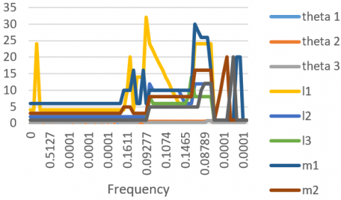
Figure 12. The data obtained with the system modeling and simulation for ${{l}_{2}}$ link
4.2 Machine learning model
The input data for model training consists of all the columns in except the last column Frequency F (Hz) which is used as output data variable. The script for model building are written in Python and using preconfigured libraries for regression analysis.Multiple linear, decision tree and random forest regression results are summarized in Table 2. The main advantages of using decision trees is the interpretability and accuracy of model tress. These results show that out of three different techniques, DTR exhibits a very good performance with R2 value > 0.97 for link 1 & 2. However, RFR shows best performance for link 3. This is because RFR gives evaluations of important variables in the regression and generates an unbiased estimate internally of the error along with progression of forest buildup.
Figure 13. The data obtained with the system modeling and simulation for ${{l}_{3}}$ link
Table 2. Machine learning result summary
|
S.No. |
Technique |
R2 value |
Details (if any) |
|
|
1. |
$\dot{\theta}_{1}$ |
Decision tree regression |
0.973552 |
-- |
|
2. |
Random forest regression |
0.944555 |
No. of estimators = 600 |
|
|
3. |
Multiple linear regression |
0.437277 |
-- |
|
|
4. |
$\dot{\theta}_{2}$ |
Decision tree regression |
0.992020 |
-- |
|
5. |
Random forest regression |
0.975063 |
No. of estimators = 600 |
|
|
6. |
Multiple linear regression |
0.355917 |
-- |
|
|
7. |
$\dot{\theta}_{3}$ |
Decision tree regression |
0.676137 |
-- |
|
8. |
Random forest regression |
0.785504 |
No. of estimators = 600 |
|
|
9. |
Multiple linear regression |
0.474677 |
-- |
|
The frequency component for various values of mass, length and angle of TLDP has been chosen from FFT analysis for further generating a machine learning model to predict frequency of angular velocity component. It is shown that machine learning algorithm is very helpful in the analysis of mechanical systems. The machine learning model predictions are in good synchronism with actual values of TLDP. This alternatively helps in prior estimation of system behavior. The same methodology can be applied to investigate other mechanical systems also in future.
This research did not receive any specific grant from funding agencies in the public, commercial, or not-for-profit sectors.
[1] Baker, G.L., Blackburn, J.A. (2005). The Pendulum: A Case Study in Physics. Oxford University Press. https://doi.org/10.1063/1.2337835
[2] Marwan, N., Romano, M.C., Thiel, M., Kurths, J. (2007). Recurrence plots for the analysis of complex systems. Physics Reports, 438(5-6): 237-329. https://doi.org/10.1016/J.PHYSREP.2006.11.001
[3] Gupta, M.K., Sharma, P., Mondal, A., Kumar, A. (2017). Visual recurrence analysis of chaotic and regular motion of a multiple pendulum system. Arabian Journal for Science and Engineering, 42(7): 2711-2716. https://doi.org/10.1007/s13369-016-2342-9
[4] Coronel-Escamilla, A., Gómez-Aguilar, J.F., López-López, M.G., Alvarado-Martínez, V.M., Guerrero-Ramírez, G.V. (2016). Triple pendulum model involving fractional derivatives with different kernels. Chaos, Solitons & Fractals, 91: 248-261. https://doi.org/10.1016/j.chaos.2016.06.007
[5] Blackburn, J.A., Yang, Z.J., Vik, S., Smith, H.J.T., Nerenberg, M.A.H. (1987). Experimental study of chaos in a driven pendulum. Physica D: Nonlinear Phenomena, 26(1-3): 385-395. https://doi.org/10.1016/0167-2789(87)90238-7
[6] Gupta, M.K., Sinha, N., Bansal, K., Singh, A.K. (2016). Natural frequencies of multiple pendulum systems under free condition. Archive of Applied Mechanics, 86(6): 1049-1061. https://doi.org/10.1007/s00419-015-1078-4
[7] Merticaru, E., Budescu, E., Iacob, R.M. (2016). Biomimetics of throwing at basketball. In IOP Conference Series: Materials Science and Engineering, 147(1): 012079. https://doi.org/10.1088/1757-899X/147/1/012079
[8] Eldukhri, E.E., Pham, D.T. (2010). Autonomous swing-up control of a three-link robot gymnast. Proceedings of the Institution of Mechanical Engineers, Part I: Journal of Systems and Control Engineering, 224(7): 825-832. https://doi.org/10.1243/09596518JSCE948
[9] Yao, Y. (2020). Numerical study on the influence of initial conditions on quasi-periodic oscillation of double pendulum system. Journal of Physics: Conference Series, 1437(1): 012093.
[10] Gupta, M.K., Bansal, K., Singh, A.K. (2014). Mass and length dependent chaotic behavior of a double pendulum. IFAC Proceedings Volumes, 47(1): 297-301. https://doi.org/10.3182/20140313-3-IN-3024.00071
[11] Sharma, P., Murali, N., Jayakumar, T. (2013). Statistical testing of temperature fluctuations for estimating thermal power in central subassembly of fast reactor. Annals of Nuclear Energy, 60: 406-411. https://doi.org/10.1016/j.anucene.2013.04.040
[12] Kaundal, V., Mondal, A.K., Sharma, P., Bansal, K. (2015). Tracing of shading effect on underachieving SPV cell of an SPV grid using wireless sensor network. Engineering Science and Technology, an International Journal, 18(3): 475-484. https://doi.org/10.1016/j.jestch.2015.03.008
[13] Jackson, B., Lorenz, R., Davis, K. (2018). A framework for relating the structures and recovery statistics in pressure time-series surveys for dust devils. Icarus, 299: 166-174. https://doi.org/10.1016/j.icarus.2017.07.027
[14] Zhou, Y., Yu, J., Wang, X. (2017). Time series prediction methods for depth-averaged current velocities of underwater gliders. IEEE Access, 5: 5773-5784. https://doi.org/10.1109/ACCESS.2017.2689037
[15] Sharma, P., Gupta, M.K., Mondal, A.K., Kaundal, V. (2017). Pattern similarity score based on one dimensional time series analysis. Journal of Pattern Recognition Research, 12(1): 1-6. https://doi.org/10.13176/11.744
[16] Zhu, Q., Azar, A.T. (Eds.). (2015). Complex System Modelling and Control Through Intelligent Soft Computations (Vol. 319). London, UK: Springer. https://doi.org/10.1007/978-3-319-12883-2
[17] Verma, V., Chauhan, P., Gupta, M.K. (2019). Disturbance observer-assisted trajectory tracking control for surgical robot manipulator. Journal Européen des Systèmes Automatisés, 52(4): 355-362. https://doi.org/10.18280/jesa.520404
[18] Edelen, A.L., Biedron, S.G., Milton, S.V., Chase, B.E., Crawford, D.J., Eddy, N., Edstrom, D., Harms, E.R., Ruan, J., Santucci, J.K., Stabile, P. (2015). Initial experimental results of a machine learning-based temperature control system for an RF gun. arXiv preprint arXiv:1511.01883.
[19] Gupta, A., Verma, V., Kumar, A., Sharma, P., Gupta, M. K., Meera, C.S. (2017). Stabilization of underactuated mechanical system using LQR technique. In Proceeding of International Conference on Intelligent Communication, Control and Devices, Springer, Singapore, pp. 601-608. https://doi.org/10.1007/978-981-10-1708-7_68
[20] Verma, V., Gupta, A., Gupta, M.K., Chauhan, P. (2020). Performance estimation of computed torque control for surgical robot application. Journal of Mechanical Engineering and Sciences, 14(3): 7017-7028. https://doi.org/10.15282/jmes.14.3.2020.04.0549
[21] Gupta, A., Mondal, A.K., Gupta, M.K. (2019). Kinematic, dynamic analysis and control of 3 DOF upper-limb robotic exoskeleton. Journal Européen des Systèmes Automatisés, 52(3): 297-304. https://doi.org/10.18280/jesa.520311