Amir Majid
© 2020 IIETA. This article is published by IIETA and is licensed under the CC BY 4.0 license (http://creativecommons.org/licenses/by/4.0/).
OPEN ACCESS
The reliability and failure rate of evaluating the lifetime extension of Ad Hoc and wireless sensor networks, are analyzed based on a probabilistic network model that assigns a failure probability from each sensor to each target zone, and when sensors are grouped in subsets, network lifetime is extended since redundancy of energizing the sensors is avoided. Theoretical formulation of reliability and failure rates of a model made of parallel sensors covering series targets, is performed, using different probability density functions (PDF) describing the performance reliability of sensors over time. The selection of the extended network lifetime depends on its reliability evaluation, which is induced as a proportionality coefficient for updating lifetime extension by adjusting the contribution of sensors energizing in cyclic time slots. Reliability is reduced with lifetime extension, but both can be increased when the number of sensors is larger than the targeted zones.
Ad hoc, failure rate, lifetime extension, probabilistic model, random lifetime variable, reliability, sensors-targets coverage, wireless sensor networks
Recent developments of ad hoc and wireless sensor networks (WSN) lead to extensive deployment of them in popular industrial and surveillant applications for sensing signals remotely, as well as controlling and monitoring facilities found in industry, health care, habitant monitoring, and military applications. These wireless networks are advantageous to wired networks due to the absence of fixed and permanent infrastructures, as well as monitoring and controlling area with limited human intervene. Yet one of the main disadvantages is power consumption, since portable energy sources of supply are limited, irreplaceable and short lived, hence the design of energy efficient systems is a challenge [1].
Preserving and maintaining sensors energy consumptions in order to prolong network lifetime, is critical to maintain targeted area coverage, since lifetime is closely associated with the consumed energy.
Previous literature shows that the coverage concept is debatable and subject to a variety of interpretations [2], as it may imply employing lossy links or deploying sensors to cover targets completely [3, 4]. In deterministic network model (DNM), specific pairs of sensor-target nodes are always connected, however, this modeling cannot guarantee full wireless network connectivity, due to transitional region probability of no coverage [5]. Energy efficient sensor-target networks are addressed in Cardei et al. [6]. Further, there are often many more lossy links in ad hoc networks than fully connected links [7]. Also with the deployment of many sensors to ensure sufficient coverage, it might aggravate large power needed to interfere with so many routing links.
Probabilistic algorithms propose organizing sensors into subsets such that each set completely covers all targets, with scheduling the time to make these subsets activated so that one set is active any time instant, hence avoid redundancy. This would conserve energy and thus prolong lifetime. many algorithms were also implemented using different methods and algorithms, such as genetic, linear programming, greedy, scheduling techniques, to name a few. Attempts are made to study the effects of geometry computations on sensor-target coverage [8], distribution of active sensors in ad hoc network [9], employing an optimum algorithm in determining sensing coverage [10], and the use of an energy-balance heuristic distributed algorithm [11]. A survey of network reliability and domination theory is attempted by Dhawan and Prasad [12].
Several reliability tools are proposed to guarantee node-to-target coverage in probabilistic algorithms, such as considering minimum probability threshold, studying transmission success ratio, i.e. node-to-node delivery ratio [13], designing a greedy based algorithm, or employing genetic optimization approaches [14], and a greedy algorithm approach [15], as well as reliable efficient energy algorithm [16]. Yet, in this study, we analyze reliability by converting the system into series-parallel topology, in which all sensors are acting in parallel to cover one target at a time, in a sequential or series pattern.
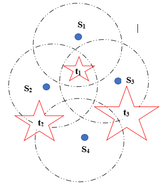
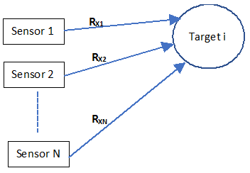
The model used in this study is a number of sensors targeting, i.e., covering a number of zones, as depicted in Figure 1 in a two-dimensional planner view. These sensor-target components can be looked as cascaded transceivers with independent probability values. That’s, each sensor covers each target with a certain probability ranging from 0 to 1. Since each target is covered by one or more sensors, full coverage can be achieved when individual sensors alone or in groups, are activated in such a way so that the total energy consumed can be decreased and hence, lifetime of the whole network is increased. The work on this model of Figure 1, is addressed in the literature with further applications [17], for simulating lifetime extension, and different senarios for lifetime extension [18]. The effect of perturbation in sensors positions in the vicinity of network targeted zones is studied [19], and the environmental effects on network lifetime extension [20].
Figure 1. Four sensors covering 3 target zones with estimated probabilities
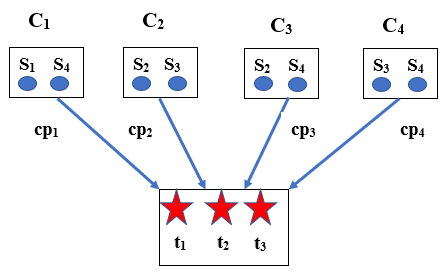
It can be noted from Figure 1, that there exists 4 possible sensor subsets or groups which cover all three target zones in full: {C1=S1,S4}, {C2=S2,S3}, {C3=S2,S4} and {C4=S3,S4}, as shown in Figure 2, Si are sensors, Ci are subsets of sensors.
Figure 2. Four sensor subsets with full target coverage, evaluated from Figure 1
In order to remove redundancies, each sensors subset is to be energized in cyclic time slots, proportional with the subset coverage probability, in an intuitive algorithm as demonstrated in Figure 3, i.e., the variable subset activation time is according to the subset value of the evaluated network probability. In the same manner, sensors are powered according to the individual sensor probability to cover corresponding targets. It is apparent that the overall subset activation times TCi for the sensor subsets will be reduced, a situation that leads to large reductions in the sensors energying times TSi.
In this work, reliability of the probabilistic network model of series-parallel sensor to target components, is analyzed in order to enhance the method used in evaluating lifetime extension. On the other hand, it’s well known that in an electrical and communication system, there is always a likelihood that over time one or more components will suddenly fail to function, that will often cause the whole system to fail, hence the failure rate of the individual components and the entire system as well, need to be evaluated accordingly. As we look into the chances that a failure might occur, this would lead to the investigation of possible designs to make the system more resilient to such failures.
Figure 3. Contributions of sensor subsets and sensors with time slots activation
Due to the probabilistic network model, the evaluation of lifetime extension is a random value. Several types of probability density functions (PDF) are considered such as exponential, Gaussian and Rayleigh, as well as with different indices and parameters. The evaluation of network reliability and failure rate, is correlated with the probability of the calculation of lifetime extension. Hence, lifetime extension is adjusted by a coefficient proportional with the evaluated reliability.
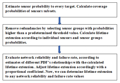
Figure 4 depicts steps and procedures performed in this study. First, probabilities are assigned for every sensor-target node, and redundancies are removed by grouping sensors that cover all target zones. Only groups that have total load coverage probabilities higher than a minimum threshold value, are selected for calculating lifetime extension. Network reliability and failure rate, are then evaluated according to assumed PDF’s relationships with time, and hence lifetime extension is adjusted with proportional coefficients.
Figure 4. Algorithms and procedure steps analyzed in this study
2.1 Reliability and failure rate
Let X be a random variable which represents the lifetime of an ad hoc and WSN network. That is, if the network is operated at time zero, X would represent the time at which the network fails. The reliability of the system RX(t) is then the probability that the network is still functioning at time t; hence
$R_{X}(t)=P_{x}(X>t)$ (1)
This means that the reliability function can be related to the cumulative distribution function (CDF) of the random variable, as,
$R_{X}(t)=1-F_{X}(t)$ (2)
where, FX(t) is the CDF. Hence the derivative of the reliability function can be related to the probability density function fX of the random variable X by
$R_{X}^{\prime}=-f_{X}(t)$ (3)
With many sensor-target components, the reliability varies with the elapsed time that the component has been functioning, and for a particular component that is still functioning at some time t, the remaining lifetime may vary differently from its initial operating time, according to a probabilistic behavior.
Failure rate is another concept used here, to describe this effect, i.e., if X is a random variable, then the failure rate function r(t) is
$r(t)=\left.f_{X \mid\{x>t\}}(x)\right|_{x=t}$ (4)
That’s, r(t)∙dt is the probability that the component will fail in the next time interval dt, given it has survived up to start time t, i.e., $P_{r}(t<x<t+d t \mid x>t)=r(t) \cdot d t$.
The failure rate can be related to the reliability function according to the conditional PDF $f_{X \mid A}(x)$ of a random variable X, as
$f_{X \mid A}(x)=\frac{d F_{X \mid A}(x)}{d x}$ (5)
in which the conditioning event A is $a \leqslant \mathrm{X} \leqslant b$, hence
$f_{X \mid\{a \leq X \leq b\}}(x)=\frac{f_{X}(x)}{\operatorname{Pr}(a \leq X \leq b)}$ (6)
in the range $a \leqslant \mathrm{X} \leqslant b$ and equal to 0 otherwise, thus
$f_{\mathrm{X} \mid\{\mathrm{x}>\mathrm{t}\}}(x)=\frac{f_{X}(t) \cdot U(x-t)}{1-F_{X}(t)}$ (7)
the denominator of the above expression is the reliability function RX(t), while the PDF in the numerator is simply $-R_{X}^{\prime}(t)$. Hence, the failure rate function evaluated at x=t, is
$r(t)=-\frac{R_{X}^{\prime}(t)}{R_{X}(t)}$ (8)
So, if the failure rate r(t) is given, then the reliability function is solved from the 1st order differential equation
$d / d t\left(R_{X}(t)\right)=-r(t) \cdot R_{X}(t)$ (9)
subject to initial conditions (I.C.) RX(0)=1, in which the general solution is
$R_{X}(t)=\exp \left[-\int_{0}^{t} r(u) d u\right] u(t)$ (10)
and since $f_{X}(t)=-R_{X}^{\prime}(\mathrm{t})$, whence the PDF of device lifetime is
$f_{X}(t)=r(t) \exp \left[-\int_{0}^{t} r(u) d u\right] u(t)$ (11)
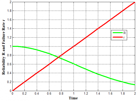
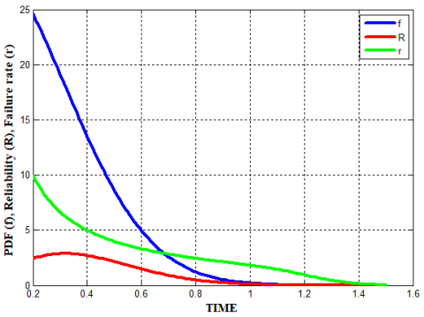
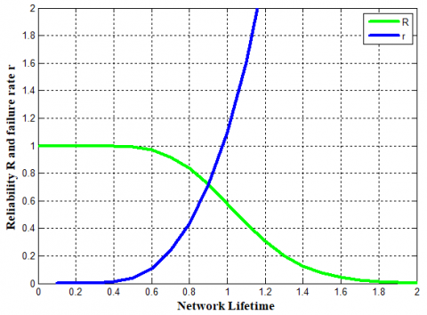
Hence, for a constant failure rate function, both the PDF of lifetime and reliability function follow an exponential manner. Figure 5 depicts the lifetime reliability function RX(t) and failure rate function r(t) for a sensor-target (S-T) component that follows a Rayleigh distribution, i.e. the pdf of random variable x=t is: fX (t)=2bt exp(-bt2) u(t), in which we assume b=0.5. That is, the depletion of device lifetime is around 50% in 5 years, yields
Figure 5. Reliability (R) and failure rate (r) of the pdf $t e^{-0.5 t^{2}}$
$R(t)=\int_{t}^{0} t e^{-0.5 t^{2}} d t=e^{-0.5 t^{2}}$ (12)
and from Eq. (8),
$r(t)=t u(t)$ (13)
As seen the reliability is an inverse exponential function of time, whereas failure rate is a linear relationship with time, and it relates closely with the lifetime PDF, as it is equal to $f_{X}(t) / R_{X}(t) .$ For example, if $\mathrm{r}(\mathrm{t})$ is a constant of value $\lambda,$ then $f_{X}(t)=t e^{\left(-\lambda t^{2}\right)} u(t), \quad$ and $\quad R(t)=-\frac{1}{2 \lambda} e^{(-\lambda t)} u(t), \quad$ that means it doesn’t matter how long the network is functioning, the failure rate is the same.
Other PDF versions are considered. Figure 6 depicts reliability and failure rate for an exponential probability density function exp(-λt), whereas Figure 7 for a Gaussian PDF, $f(t)=k e^{\left(-\lambda t^{2}\right)}$. Note that the failure rate for exp(-λt) is constant over time.
Figure 6. PDF (f), reliability (R) and failure rate (r) for the PDF $e^{-0.5 t}$
Figure 7. PDF (f), reliability (R) and failure rate (r) of the pdf $k_{1} e^{-k_{2} t^{2}}$
We shall adopt throughout in this study the Raleigh random [21], resembling the lifetime of an actual sensors network covering a number of target zones, as initially at installation time, the probability of lifetime is low or unexpected, but soon after it functions with increasing value to a maximum value, and then dropping exponentially with time
2.2 Ad hoc and WSN reliability
Consider an ad hoc network comprising N sensor-M target components, with each sensor has a lifetime probability described by a Rayleigh PDF in an independent manner to each other. Hence, the lifetime reliability to cover any target is evaluated with all sensors operated or energized in parallel for the same target. That is, the system will be functioning as long as any one of the sensors is functional, as depicted in Figure 8, that’s
Figure 8. Multiple sensors covering one target zone with different reliabilities, RX
$R(t)=P_{r}\left(\left\{X_{1}>t\right\} \cup\left\{X_{2}>t\right\} \cup . . \cup\left\{X_{N}>t\right\}\right)$ (14)
where $, R(t)$ is the overall reliability, $X_{n}, n=1, N$ are sensors lifetime random variables and the coverage system will fail only if all individual sensors fail, and with $P_{r}(X \leq t)$ equal to $1-R_{X}(t),$ this leads to
$P_{r}(X \leq t)=P_{r}\left(\left\{X_{1} \leq t\right\} \cup\left\{X_{2} \leq t\right\} \cup . . \cup\left\{X_{N} \leq t\right\}\right.$ (15)
which is equivalent to the relationship: $P_{r}\left(X_{1} \leq t\right) \cap P_{r}\left(X_{2} \leq\right.t) \cap . \cap P_{r}\left(X_{N} \leq t\right)=\left(1-R_{X_{1}}(t)\right)\left(1-R_{X_{2}}(t)\right) \ldots(1-\left.R_{X_{N}}(t)\right),$ hence
$R_{X}(t)=1-\prod_{n=1}^{N}\left(1-R_{X_{\eta}}(t)\right)$ (16)
and again from Eq. (8)
$r(t)=\frac{1-R_{X}(t)}{R_{X}(t)} \sum_{n=1}^{N}\left\{\frac{R_{X}^{\prime} x_{n}(t)}{1-R_{X_{n}}(t)}\right\}$ (17)
This can be rearranged as
$r(t)=\left(\frac{1}{R_{X}(t)}-1\right) \sum_{n=1}^{N}\left\{\frac{r_{n}(t)}{\frac{1}{R_{X_{n}}(t)}-1}\right\}$ (18)
Figure 9 demonstrates same number of the previous network sensors covering several target zones simultaneously, which can be looked at as a series-parallel components, in which parallel sensors covering an entire network targets in a series sequence, i.e. a network can be said to be completely covered only when all targets zones are covered.
Figure 9. N parallel sensors covering M series targets in sequence
The reliability of one sensor covering a number of targets, is therefore the multiplication of reliability of all sensor covering each target, since they are generally independent. This is an assumption adopted in this study, else the joint reliability of multiple random variables must be implemented, which can be complicated for a large number of sensors.
Therefore, it is possible to calculate the reliability and failure rate functions of the entire sensor-target system by considering all affected targets interconnected in series as demonstrated in Figure 9, so that if any individual fails, the whole system fails. Let’s define now Y to be the random variable representing the lifetime of the system comprising N random variables; $X_{n}, n=1 \ldots N$ , in which all S-T components fail independently, hence
$Y=\min \left(X_{1}, X_{2}, \ldots, X_{N}\right)$ (19)
furthermore,
$R_{Y}(t)=P_{r}(Y>t)=P_{r}\left(\left\{X_{1}>t\right\} \cap\left\{X_{2}>t\right\} \cap . .\right)$ (20)
which is also equal to $P_{r}\left(X_{1}>t\right) P_{r}\left(X_{2}>t\right) . .,$ and hence $R_{Y}(t)=R_{X_{1}}(t) R_{X_{2}}(t) . .,$ then using $(8),$ reveals
$r(t)=\frac{-R_{Y}^{\prime}(t)}{R_{Y}(t)}=\frac{-\frac{d}{d t}\left[R_{X_{1}} \cdot\cdot\right]}{R_{X_{1}} R_{X_{2}} \cdot\cdot}$ (21)
that’s,
$r(t)=-\sum_{n=1}^{N} \frac{R_{X_{n}}^{\prime}}{R_{\mathrm{Y}}}=\sum_{n=1}^{N} r_{n}(t)$ (22)
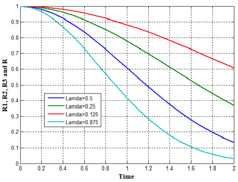
where, rn(t) is the failure rate function of the nth sensor-target component, so for a series connection, the reliability function of system is the product of the reliability functions of each component and the failure rate function is the sum of the failure rate functions of all individual components. Figure 10 depicts 3 interconnected system in series, with failure rate values, $\lambda=\left[\begin{array}{ll}0.5, & 0.25,0.125,0.875\end{array}\right],$ which is equal to $\mathrm{r},$ and reliability values, $R_{1}=e^{-0.5 t^{2}}, R_{2}=e^{-0.25 t^{2}}, R_{3}=e^{-0.125 t^{2}} R_{\text {total}}=e^{-0.875 t^{2}},$ which yields that the total failure rates equals the sum of individual failure rates.
Figure 10. Reliability of 3 interconnected systems in series, with their total, for lamda, λ=[0.5, 0.25, 0.125, 0.875]
Different sensor-target components have different failure rates that behave in different manners. Here, one can imagine that such devices might have decreasing or increasing failure rate functions at part of their lifetimes, while others have failure rates which remain constant with time, in which the latter is assumed in this study.
For N components, each with a constant failure rate, $r_{n}(t)=\lambda_{n}, n=1 \cdot\cdot N$. Note that a constant failure rate corresponds to exponentially reliability function
$R_{X_{n}}(t)=\exp \left(-\lambda_{n} t\right) u(t)$ (23)
$R_{X}(t)=\prod_{n=1}^{N} R_{X_{n}}(t)=\prod_{n=1}^{N} \exp \left(-\lambda_{n} t\right) u(t)$ (24)
with $\lambda=\left[\lambda_{1}, \lambda_{2}, \cdot\cdot \lambda_{N}\right]$, which yields
$R_{X}(t)=\exp \left[-\left\{\sum_{n=1}^{N} \lambda_{n}\right\} t\right] u(t)$ (25)
And
$r(t)=\sum_{n=1}^{N} r_{n}(t)=\sum_{n=1}^{N} \lambda_{n}$ (26)
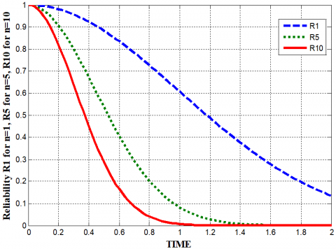
Figure 11 depicts a case study with different number of targets, namely one, 5 and 10, in which it can be noted that reliability drops more, yet it is not significant beyond numbers around 5 targets.
Now, when a number of sensors covering the same target zone, then the reliability of the whole system is increased due to components connected in parallel, that’s,
$R_{X}(t)=\left\{1-\prod_{n=1}^{N}\left[1-\exp \left(-\lambda_{n} t\right)\right]\right\} u(t)$ (27)
and
$r(t)=\frac{\prod_{n=1}^{N}\left[1-\exp \left(-\lambda_{n} t\right)\right]}{1-\prod_{n=1}^{N}\left[1-\exp \left(-\lambda_{n} t\right)\right)} \sum_{n=1}^{N} \frac{\lambda_{n}}{\exp \left(\lambda_{n} t\right)-1}$ (28)
Figure 11. Reliabilitities R1, R5, R10, of one sensor covering n number of targets; n=1, 5 and 10
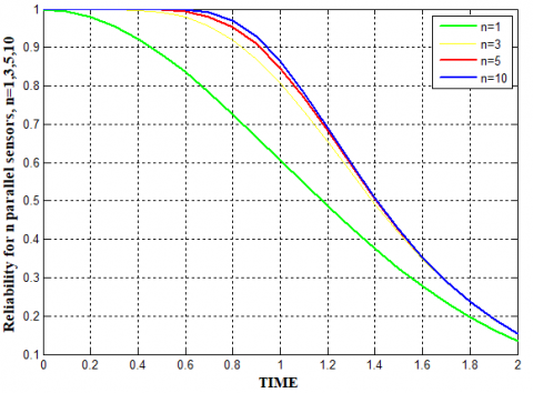
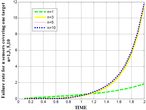
With these equations, the reliability and failure rate of n sensors, with n=1, 3, 5 and 10, covering one target zone area is simulated as shown in Figure 12. As seen, reliability is improved with number of parallel sensors n increasing, yet there will be no significant change more when n>5. Figure 13 depicts the same parallel components effect on the failure rate, which decreases as number of parallel components increase, but eventually increases when lifetime is more than 1.2.
Figure 12. Reliabilities of n sensors covering one target zone for n=1, 3, 5, 10
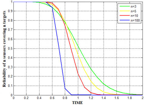
The reliability of the entire network comprising a number of sensors covering same number of targets is depicted in Figure 14, where it can be noted that reliability drops as this number is increasing. We can deduce that reliability is reduced to zero with large number of sensors equals to number of targets.
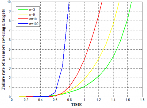
Similarly, Figure 15 shows the failure rate variation with n, which increases sharply. Intuitively, failure rate and reliability will be reduced in cases of large number of sensors-targets networks, when the number of sensors is not larger than number of targets.
Figure 13. Failure rates of multiple sensors covering one target zone for n=1, 3, 5 and 10
Figure 14. Reliability of n sensors covering n target zones, for n=3, 5, 10 and 100
Figure 15. Failure rate of n sensors covering n target zones, for n=3, 5, 10 and 100
3.1 Algorithm of the used method
A flow chart, that is listed in the Appendix, depicts steps used in the used algorithm, such as sensors subsetting and removal of redundancies, evaluating relibility and failure rates of the selected sensor subsets, contributions of each sensor energizing, in supplying the total load demand.
In the first step, in a network with N sensors covering M targets, sensors subsets that cover all target zones are selected according to sensor-target individual probabilities. Subsets coverage probabilities that are larger than a predefined threshold value is selected [1].
In the second step, the relibility and failure rate of each of the selected sensors subset to all target zones, are calculated as depicted in Eq. (21), (21), (27) and (28).
In the third step, the joint probabilities are calculated with amount of variations in the mean value of these probabilities, a predefined threshold is introduced, in which only joint probabilities larger than a predefined threshold value are selected. This would control redundancies on the used number of sensors. Also, the sharing percentage of each sensor combination are calculated for the total load demand.
In the third step, the overall network joint reliability for the calculated value of time extension in step 1, is evaluated. We compare this value with an assigned value needed for the overall network reliability. Then, we adjust the lifetime extension accordingly, in which normally it is reduced when the required reliability is higher than the calculated one. This step constitutes the main work in this research.
Finally, we calculate the sharing percentage of every sensor subset, as well as contribution percentage each sensor within the subsets. Hence, each network sensor will be energized according to its sharing percentage in all combinations.
3.2 Case study
The above analysis is applied on a case study of a wireless ad hoc and sensor network comprised of 4 sensors covering 3 target zones, denoted 4S-3T, with both reliability and failure rate calculated against network lifetime extension, which is evaluated according to the algorithm depicted in the Appendix flowchart. This as shown in Figure 16, in which as expected, the reliability decreases with larger network lifetimes, and failure rate increases exponentially with lifetime. Here we assumed a Rayleigh PDF relationship with sensor lifetime. Other PDF relationships can also be considered depending on the nature of sensors lifetimes. It is noted that reliability varies inversely with referenced lifetime values in the range between 0.6-1.6, whereas failure rates increase heavily in the same range, hence, a comprised value of lifetime extension is to be considered for a proper network operation.
Here, we need first to prolong network lifetime with assumed probability values of sensors-to-targets, that are shown in Table 1.
In order to follow terminations [1] and to compare results, we shall use here the term of failure probability (FP), rather than probability (P), in which FP=1-P, and coverage failure probability (CFP) for coverage probability (CP). Note, that this assumption of sensor-target failure probability has been exaggerated to address worse scenario.
Next, to extend network lifetime, redundancies in sensors contributions are removed, by grouping sensors in subsets, in which each subset covers all targets with a certain coverage failure probability. Using an implemented algorithm with above table data, we obtain the following nine subsets together with the values of their corresponding network coverage failure probabilities [20], as depicted in Table 2.
Figure 16. Reliability (R) and failure rate (r) of a 4S-3T network
Figure 17. Reliability (R) of 4S-3T network with four selected sensor subsets
Table 1. Sensor-target probability (FP)
|
Sensor-Target |
S1-T1 |
S2-T1 |
S2-T2 |
S3-T1 |
S3-T3 |
S4-T2 |
S4-T3 |
|
FP |
0.7 |
0.3 |
0.5 |
0.2 |
0.9 |
0.7 |
0.4 |
|
SS |
{1,4} |
{1,2,3} |
{1,2,3,4} |
{1,2,4} |
{1,3,4} |
{2,3} |
{2,4} |
{2,3,4} |
{3,4} |
|
CFP |
0.946 |
0.952 |
0.601 |
0.691 |
0.834 |
0.953 |
0.727 |
0.609 |
0.846 |
|
SS |
{1,2,3,4} |
{1,2,4} |
{2,4} |
{2,3,4} |
|
CFP |
0.601 |
0.691 |
0.727 |
0.609 |
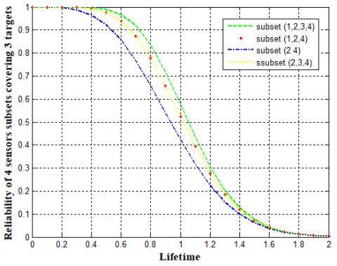
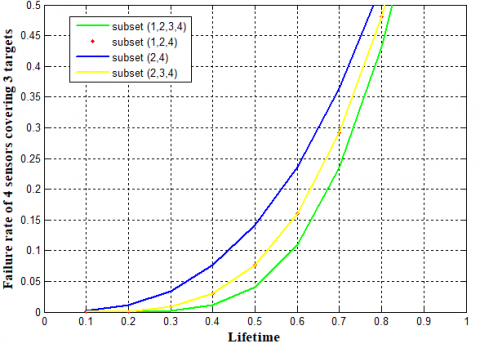
The reliability and failure rate of these 4 subsets are then evaluated according to above reliability and failure rate analysis. The following curves in Figure 17 display the reliability of each sensor subset. It can be noted that with sensor subset {1, 2, 3, 4} of four sensors, the reliability is increased compared to other subsets, whereas the failure rate is decreased (Figure 18).
Figure 18. Failure rates of 4S-3T network with four selected sensor subsets
It is apparent that reliability and failure rate values are variable with each activating subset or groups of sensors acting a time. With each subset having different coverage probability, we can realize that the calculation of lifetime extension is variable and dependent on the extend of the evaluated reliability.
It is intended to evaluate the reliability and failure rate of each sensor subset that satisfies a minimum coverage failure probability constraint for the entire network. By this method, we extend network lifetime and consequently energy, with the reliability condition. The reliability of each sensor subset is used to adjust the time slot activation of each sensor subset, as demonstrated in Figure 3. Intuitively, a proportional constant, based on maximum reliability of the subsets for a certain lifetime value, is merely multiplied by the time slot of each subset contribution to estimate the net energizing time for each subset, as depicted in Table 4.
Table 4. Sensors subsets time slot contribution
|
Subset SS |
{1,2,3,4} |
{1,2,4} |
{2,4} |
{2,3,4} |
|
Coverage CFP |
0.601 |
0.691 |
0.727 |
0.609 |
|
Reliability R |
0.290 |
0.227 |
0.199 |
0.285 |
|
Time slot A |
0.590 |
0.530 |
0.430 |
0.530 |
|
Time slot B |
0.329 |
0.231 |
0.164 |
0.290 |
Hence sensor subsets are adjusted for their coverage failure probability as well as reliability. Table 5 depicts the adjusted contribution of each sensor share in the energizing time slot.
Using the intuitive scheme demonstrated in Figure 3, for determining cyclic time slot sharing, it reveals that sensor 2 is energized maximum for 41.41% of the total cyclic time, whereas sensor 1 is energized minimum of 11.92% of the time. This condition would offer maximum reliability as well as network time extension of 2.8574 of the normalized time.
Table 5. Sensors time slot contribution
|
Subset SS |
{1,2,3,4} |
{1,2,4} |
{2,4} |
{2,3,4} |
|
Subset contribution |
0.3298 |
0.2317 |
0.1646 |
0.2906 |
|
S1 Timing =0.1192 |
0.0606 |
0.0586 |
|
|
|
S2 Timing =0.4142 |
0.1069 |
0.0983 |
0.0940 |
0.1150 |
|
S3 Timing =0.1665 |
0.0802 |
|
|
0.0863 |
|
S4 Timing =0.3107 |
0.0802 |
0.0737 |
0.0705 |
0.0863 |
It has been considered that PV sets are supplying in parallel any single load center, i.e. in parallel, whereas repeating this analysis in sequence for all load centers, that’s parallel-series analysis. Due to the concept of network reliability, series-parallel reliability analysis has not been considered in this study.
Due to large computational time, only small number of PV sets and load centers are considered. For example, for 10 PV sets, there could be a maximum of 1023 different combinations to analyses, and if computational time for a single combination, say 3 sec, it might take approximately an hour to complete calculation.
The significant of this study is the correlation between lifetime extension using power coverage probability, and the reliability of evaluating this lifetime extension.
There were not many algorithms to consider network reliability [1], reliable lifetime was defined as equal to current active sensor cover’s failure probability times current network lifetime, and simulations were made for different predefined threshold values (denoted as α in this work). Earlier, there were previous attempts to associate reliability with genetic algorithm, which is different from this work, by defining the minimum node-to-node delivery ratio between any pair of dominators, to be within a predefined threshold value. In this study, we did not compare the probabilistic model that is implemented in this study with other models used for extending network lifetime.
The reliability and failure rate of an entire wireless ad hoc and sensor network are evaluated based on a Rayleigh PDF relationship describing one sensor coverage of one target zone with a certain probability, in which a probabilistic network model with series-parallel components concept, is employed.
Theoretical analyses of parallel sensors acting on series targets are demonstrated for different sizes of networks. The evaluated reliability values are augmented with the network coverage failure probabilities, in order to find the most reliable subsets that can be energized for the reliable lifetime extension that has been evaluated earlier.
A case study of 4 sensors covering 3 targets is simulated for both lifetime extension and reliability constraint, as well as contribution of sensors energizing in cyclic time slots, have been calculated. A compromise between reliability and lifetime extension is made, and as a result, differentiation between network coverage probability and the reliability of network lifetime extension, has been attempted.
Extra investigation would be useful to study other types of PDF relationships describing sensors lifetimes, method of adjusting lifetime extension with reliability, as well as the intuitive scheme used in determing sensors and sensor subsets time sharing.
|
Ci Si TCi TSi X, Y RX(t) Pr M N FX(t) r(t) Ri f(t) FP CFP SS CP u(t) |
sensor subset or group sensor subset coverage time slot sensor coverage time slot random variables reliability of X probability number of targets number of sensors CDF of X failure rate PDF relationships time function failure probability coverage failure probability sensor subset coverage probability unit time function |
|
Greek symbols |
|
|
λi ∩ ∪ |
failure rate value AND OR |
|
Subscripts |
|
|
x y z i n N |
value of random variable X value of random variable Y value of random variable Z index index maximum index |
[1] He, J., Ji, S., Pan, Y., Li, Y. (2011). Reliable and energy efficient target coverage for wireless sensor networks. Tsinghua Science and Technology, 16(5): 464-474. https://doi.org/10.1016/S1007-0214(11)70066-9
[2] Akyildiz, I.F., Su, W., Sankarasubramaniam, Y., Cayirci, E. (2002). A survey on sensor networks. IEEE Communications Magazine, 40(8): 102-114. https://doi.org/10.1109/MCOM.2002.1024422
[3] Slijepcevic, S., Potkonjak, M. (2001). Power efficient organization of wireless sensor networks. IEEE International Conference on Communications. Conference Record (Cat. No.01CH37240), Helsinki, Finland, pp. 472-476. https://doi.org/10.1109/ICC.2001.936985
[4] Kar, K., Banerjee, S. (2003). Node placement for connected coverage in sensor networks. Modeling and Optimization in Mobile, Ad Hoc and Wireless Networks.
[5] Yan, T., He, T., Stankovic, J.A. (2003). Differentiated surveillance for sensor networks. SenSys '03: Proceedings of the 1st International Conference on Embedded Networked Sensor Systems, pp. 51-62. https://doi.org/10.1145/958491.958498
[6] Cardei, M., Thai, M. T., Li, Y., Wu, W. (2005). Energy-efficient target coverage in wireless sensor networks. Proceedings IEEE 24th Annual Joint Conference of the IEEE Computer and Communications Societies., Miami, FL, pp. 1976-1984. https://doi.org/10.1109/INFCOM.2005.1498475
[7] Wang, Y.C., Hu, C.C., Tseng, Y.C. (2007). Efficient placement and dispatch of sensors in a wireless sensor network. IEEE Transactions on Mobile Computing, 7(2): 262-274. https://doi.org/10.1109/TMC.2007.70708
[8] Wang, S.Y., Shih, K.P., Chen, Y.D., Ku, H.H. (2010, April). Preserving target area coverage in wireless sensor networks by using computational geometry. 2010 IEEE Wireless Communication and Networking Conference, Sydney, NSW, pp. 1-6. https://doi.org/10.1109/WCNC.2010.5506575
[9] Shih, K.P., Chen, Y.D., Chiang, C.W., Liu, B.J. (2006). A distributed active sensor selection scheme for wireless sensor networks. 11th IEEE Symposium on Computers and Communications (ISCC'06), Cagliari, Italy, pp. 923-928. https://doi.org/10.1109/ISCC.2006.7
[10] Zhang, H., Wang, H., Feng, H. (2009). A distributed optimum algorithm for target coverage in wireless sensor networks. 2009 Asia-Pacific Conference on Information Processing, Shenzhen, pp. 144-147. https://doi.org/10.1109/APCIP.2009.172
[11] Zhang, H. (2009). Energy-balance heuristic distributed algorithm for target coverage in wireless sensor networks with adjustable sensing ranges. 2009 Asia-Pacific Conference on Information Processing, Shenzhen, pp. 452-455. https://doi.org/10.1109/APCIP.2009.247
[12] Dhawan, A., Prasad, S.K. (2009). A distributed algorithmic framework for coverage problems in wireless sensor networks. International Journal of Parallel, Emergent and Distributed Systems, 24(4): 331-348. https://doi.org/10.1080/17445760902720008
[13] Agrawal, A., Barlow, R.E. (1984). A survey of network reliability and domination theory. Operations Research, 32(3): 478-492. https://doi.org/10.1287/opre.32.3.478
[14] Wang, J., Niu, C., Shen, R. (2009). Priority-based target coverage in directional sensor networks using a genetic algorithm. Computers & Mathematics with Applications, 57(11-12): 1915-1922. https://doi.org/10.1016/j.camwa.2008.10.019
[15] Zhang, H.W., Wang, H.Y., Feng, H.C., Liu, B., Gui, B.X. (2009). A heuristic greedy optimum algorithm for target coverage in wireless sensor networks. 2009 Pacific-Asia Conference on Circuits, Communications and Systems, Chengdu, pp. 39-42. https://doi.org/10.1109/PACCS.2009.87
[16] He, J., Ji, S.L., Pan, Y., Li, Y.S. (2014). Reliable and energy efficient target coverage for wireless sensor networks. Tsinghua Science & Technology, 16(5): 464-474. https://doi.org/10.1016/S1007-0214(11)70066-9
[17] Majid, A.J. (2015). Matlab simulations of ad hoc sensors network algorithm. International Journal on Recent and Innovation Trends in Computing and Communication, 3(1): 288-293. https://doi.org/10.17762/ijritcc2321-8169.150159
[18] Majid, A.J. (2015). Algorithm with simulations of network sensors lifetime and target zones coverage. Asian Journal of Mathematics and Computer Research, 6(3): 213-224.
[19] Majid, A.J. (2015). Maximizing Ad hoc network lifetime using coverage perturbation relaxation algorithm. WARSE International Journal of Wireless Communication and Network Technology, 4(6): 77-83.
[20] Majid, A. (2019). Shadowing and fading environmental effects on lifetime extension of ad hoc wireless networks. 2019 International Conference on Electrical and Computing Technologies and Applications (ICECTA), Ras Al Khaimah, United Arab Emirates. http://dx.doi.org/10.1109/ICECTA48151.2019.8959757
[21] Scott, M., Childers, D. (2012). Engineering Applications: Reliability and Failure Rates, Probability and Random Processes. Academic Press.