Kotha Gangadhar | Dhanekula Naga Bhargavi | Venkata Subba Rao Munagala*
© 2020 IIETA. This article is published by IIETA and is licensed under the CC BY 4.0 license (http://creativecommons.org/licenses/by/4.0/).
OPEN ACCESS
In the current work boundary layer flow of Casson fluid over a stretched sheet is considered to analyze the heat transfer analysis in presence of viscous dissipation. The study of Casson fluid is the best study to analyze the nature of non-Newtonian fluid. The set ordinary equations are derived from the governing equations of the flow along with boundary conditions. The transformed coupled ordinary differential equations are solved numerically by using the spectral relaxation method. Later the numerical solutions are compared with exact solutions. The consequences of governing parameters on dimensionless quantities like velocity, temperature, friction factor and local Nusselt numbers are shown and discussed. Here the result shows that the Casson fluid has a propensity to decrease the velocity of the fluid due to its higher viscidness. And the fluid of relatively small Prandtl number has high temperature in the occurrence of viscous dissipation. Applications of such type of problems are obtained in the control of complex fluid materials significant to energy and biomedical systems.
SRM, exact solutions, Casson fluid, nonlinear stretching sheet, viscous dissipation
In the view of both theoretical and applied points the fluid flow over a stretching sheet has more importance in the plastic engineering and metallurgy. Consequently, the study of stretching sheet flow has importance in the applications of paper counting production, manufacturing of aluminum bottle process, illustration of copper wires, metallurgical processes, spiraling of fibers, plastic and rubber sheets manufacture, film coating and crystal growing etc. In the development of extrusion worth of the final product is depends on the percentage of stretching along with the occurring heating or cooling. Therefore, in several industrial processes the fluid flow and heat transfer over the stretching sheet have a realistic importance.
Crane [1] conducted a study to examine the flow because of the stretching of a sheet. Further, Sakiadis [2] initiated the thought of boundary layer flow over a moving surface. Later, Tsou et al. [3] analyzed the momentum and heat transfer aspects in both analytical and experimental method over a stretching surface. After that, a number of authors, Noor et al. [4], Prasannakumara et al. [5], Bilal et al. [6] broadened the notion of a stretching sheet for different fluid models. They are concluded that there are numerous numbers of applications in polymer industry. Further, Mabood et al. [7] analyzed the study of time-independent flow of non-Newtonian fluids. Casson fluid can be assumed as a shear thinning model and at zero shear rate it having infinite viscosity , moreover , there is no flow at below the yield stress.
As of we know that Casson model is the one of the well-known rheological form to characterize the nature of non-Newtonian fluids along with the yield stress [8]. For viscous suspensions of cylindrical particles the Casson fluid form is developed [9]. Why Casson fluid has great importance means this model has nonlinear yield-stress-pseudo plastic nature, apart from it describes the various types of suspensions. Examples for such type of fluids are blood [10], chocolate [11], and xanthan gum solutions [12]. According to the authors Kirsanov et al. [13], Joye [14] comparatively general Herschel-Bulkley model gives a better flow data with power-law dependence for the yield stress. Bird et al. [15], Wilkinson [16] Rheological fluids are chocolate , blood and Casson models. This form appears to vigorous the nonlinear conduct of yield stress-pseudo plastic fluids quite well, and its prominence developed since its presentation in 1959. It is moderatively easy to utilize, and it is firmly identified with the Bingham form Bird et al. [15], Wilkinson [16] which is in all aspects broadly utilized to depict the flows of slurries, suspensions, ooze, and other rheological complex fluids Churchill [17]. Later Boyd, Buick, and Green [18] they utilized model of Casson fluid is utilized to study the steady as well as oscillatory blood flow. As of late, a flow of boundary-layer of a Casson fluid over groups of various geometries was contemplated by numerous authors.In this connection, Nadeem, Haq, and Lee [19] contemplated about the MHD flow of exponentially shrinking sheet by considering the Casson fluid as working model. Later Kumari et al. [20] examined the peristaltic pumping of an MHD Casson fluid in an inclined channel. Further Sreenadh, Pallavi, and Satyanarayana [21] considered a Casson fluid flow all the way through an inclined tube of a non uniform cross section. Mukhopadhyay et al. [22] well thought out an unsteady 2D flow of a non-Newtonian fluid by means of a prescribed surface temperature. A detail note is presented on steady fully-developed laminar flow of Casson fluid [23]. In perspective on the non-Newtonian nature of blood in vessels and filtration/assimilation property of the dividers, Further Saqib et al. [24] got the Laplace transformation strategy for the Casson liquid over a boundless swaying plate.
The flow of heat transfer in together viscous and elastic type of fluid characteristics over a stretching sheet through power law of surface temperature was examined by Vajravelu and Roper [25] while Alinejad et al. [26] explored this spectacle in a viscous fluid over a non-linear stretching sheet by including the effects of heat dissipation. Zaimi et al. [27] investigated the fluid flow due to a permeable stretching sheet with viscous effect. Later Dhanai et al. [28] prolong the work of Zaimi together with the MHD flow with viscous dissipation effect. Mobood et al. [29] also considered the boundary layer flow with heat and mass of an electrically conductively water based nanofluid of a nonlinear stretching sheet through viscous dissipation effect. Goyal and Bhargava [29] premeditated the triple diffusive boundary layer flow of nanofluid over a nonlinear stretching sheet. Later Shen et al. [30], Jat and Chaudhary [31] examined the MHD boundary layer flow with heat transfer for stagnation point over a stretching sheet with and without viscous dissipation and Joule heating. Dessie and Kishan [32] considered the boundary layer flow with heat transfer over a stretching sheet embedded in a porous medium by enchanting the effect of viscous dissipation and heat source/sink in the presence of uniform magnetic field.
By the above all motivated investigations, the present research is concentrated on the laminar boundary layer flow of Casson fluid along with heat transfer treatment in the occurrence of viscous dissipation. By utilizing the appropriate transformations order of the ordinary differential equations relating to the momentum and energy equation are reduced and then by using spectral relaxation method these equations can be solved numerically. Later obtained numerical solutions are exhibit in graphs and tables to study the variations of various values of the dimensionless parameters which are used in this problem. The investigation of the results shows that the flow field is significantly affected by the leading parameters. A very important industrial application, like estimation of the skin friction is also presented in this analysis. Hence here the investigation is expecting that the results which we obtained are not only useful for applications but also used as a complement to the earlier studies.
Let us consider two-dimensional, steady, boundary-layer flow, incompressible, viscous fluid, over a sheet. It coincides at y=0. The region flow refers to y>0. Two equal and opposite forces are applied in the direction of x component. The sheet has a velocity uw(x)=axn by means of fixed origin location, where n is refer to nonlinearity parameter, if n=1 then the case is refer linear case and n ≠1 is refer nonlinear case, a refer constant and it considered as a>0. The rheological equation for Casson fluid is given below.
$\tau_{i j}=\left\{\begin{array}{l}2\left(\mu_{B}+\frac{p_{y}}{\sqrt{2 \pi}}\right) e_{i j}, \pi>\pi_{c} \\ 2\left(\mu_{B}+\frac{p_{y}}{\sqrt{2 \pi_{c}}}\right) e_{i j}, \pi<\pi_{c}\end{array}\right.$ (1)
where, π refer to the rate of deformation of product of component and it can be defined as π=eij eij, πc is refer to critical value of the product non – Newtonian fluid model, $\mu_{B}$ is refer to plastic dynamic viscosity, and py is refer to fluid yield stress. Tw is referring to temperature at the wall and it can be assumed that this value is constant at the stretching surface. The ambient temperature is referring to T∞ at this position y is tending to infinity. Moreover, boundary condition for Newtonian heating condition is involved in energy equation. The physical sketch of present model is shown in Figure 1.
Figure 1. Physical model and coordinate system
The governing equations of momentum and thermal energy can be written as, Mukhopadhyay [33].
$\frac{\partial u}{\partial x}+\frac{\partial v}{\partial y}=0$ (2)
$u \frac{\partial u}{\partial x}+v \frac{\partial u}{\partial y}=v\left(1+\frac{1}{\beta}\right) \frac{\partial^{2} u}{\partial y^{2}}$ (3)
$u \frac{\partial T}{\partial x}+v \frac{\partial T}{\partial y}=\alpha \frac{\partial^{2} T}{\partial y^{2}}+\frac{\mu}{\rho c_{p}}\left(1+\frac{1}{\beta}\right)\left(\frac{\partial u}{\partial y}\right)^{2}$ (4)
where, u and v are referring to velocity segments in the direction of x and y correspondingly, v is refer to viscosity of kinematic, μ is refer to viscosity of the fluid, α=k/ρcp is refer to thermal diffusivity, k is refer to the thermal conductivity, ρ is refer to fluid density, cp is refer to specific heat at constant pressure, β=μB √(2πc)/py is refer to Casson fluid parameter.
The following are the boundary conditions:
$u=u_{w}=a x^{n}, v=0, T=T_{w},$ at $y=0,$ (5)
$u \rightarrow 0, T \rightarrow T_{\infty},$ as $y \rightarrow \infty$ (6)
Here, a is refer to constant and it can be taken as a>0, n is referring to power law numbe it can be used to measure the velocitof the stretching surface, hs is heat transfer parameter.
Let Ψ be the stream function of this study and it satisfies the condition $u=\frac{\partial \Psi}{\partial y}$ and $v=-\frac{\partial \Psi}{\partial x}$ by this defined function of the Eqns. (2)-(4) can be written as follows:
$\frac{\partial \Psi}{\partial y} \frac{\partial^{2} \Psi}{\partial x \partial y}-\frac{\partial \Psi}{\partial x} \frac{\partial^{2} \Psi}{\partial y^{2}}=v\left(1+\frac{1}{\beta}\right) \frac{\partial^{3} \Psi}{\partial y^{3}}$ (7)
$\frac{\partial \Psi}{\partial y} \frac{\partial T}{\partial x}-\frac{\partial \Psi}{\partial x} \frac{\partial T}{\partial y}=\alpha \frac{\partial^{2} \mathrm{T}}{\partial y^{2}}+\frac{\mu}{\rho c_{p}}\left(1+\frac{1}{\beta}\right)\left(\frac{\partial^{2} \Psi}{\partial y^{2}}\right)^{2}$ (8)
Consequently boundary conditions are follows as:
$\frac{\partial \Psi}{\partial y}=u_{w}=a x^{n}, \frac{\partial \Psi}{\partial x}=0, T=T_{w},$ at $y=0$ (9)
$\frac{\partial \Psi}{\partial y} \rightarrow 0, T \rightarrow T_{\infty}, \quad$ as $\quad y \rightarrow \infty$ (10)
The following are the similarity transformations:
$\Im =y\sqrt{\frac{a\left( n+1 \right)}{2v}}{{x}^{\frac{n-1}{2}}},\,\Psi =\sqrt{\frac{2va}{m+1}}{{x}^{\frac{n+1}{2}}}f\left( \Im \right),\,u=a{{x}^{n}}{f}'\left( \Im \right)$ (11)
$v=-\sqrt{av\frac{n+1}{2}}{{x}^{\frac{n-1}{2}}}\left[ f\left( \Im \right)+\frac{n-1}{n+1}\Im {f}'\left( \Im \right) \right],\,\theta \left( \Im \right)=\frac{T-{{T}_{\infty }}}{{{T}_{w}}-{{T}_{\infty }}}$ (12)
From the above assumptions Eqns. (7)-(8) can be written as:
$\left(1+\frac{1}{\beta}\right) \frac{\partial^{3} f}{\partial \mathfrak{J}^{3}}+f \frac{\partial^{2} f}{\partial \mathfrak{J}^{2}}-\frac{2 n}{n+1}\left(\frac{\partial f}{\partial \mathfrak{J}}\right)^{2}=0$ (13)
$\frac{\partial^{2} \theta}{\partial \Im^{2}}+\operatorname{Pr} f \frac{\partial \theta}{\partial \mathfrak{J}}+\operatorname{Pr} E c\left(\frac{\partial^{2} f}{\partial \mathfrak{J}^{2}}\right)^{2}=0$ (14)
Consequently boundary conditions are follows as:
$f(\mathfrak{I})=0, \frac{\partial f}{\partial \mathfrak{J}}=1, \theta(\mathfrak{I})=1$ at $\mathfrak{I}=0$ (15)
$\frac{\partial f}{\partial \Im}=0, \quad \theta(\mathfrak{I})=0 \quad$ as $\mathfrak{I} \rightarrow \infty$ (16)
The physical parameters which are involved in the present flow are defined as: $\operatorname{Pr}=\frac{v}{\alpha}, \mathrm{Ec}=\frac{u_{w}^{2}}{c_{p}\left(T_{w}-T_{\infty}\right)}$.
Here, Pr is the parameter representing the Prnadtl number and Ec is the parameter for the viscous dissipation parameter (Eckert number).
Thereafter for nonlinear stretching case proposed numerical technique is applied to solve.
In this present analysis, flow quantities like, local skin friction coefficient Cfx and Nusselt number Nux, and they are follows:
$C_{f x}=\frac{\mu}{\rho u_{w}^{2}}\left(\frac{\partial u}{\partial y}\right)_{y=0}, N u_{x}=\frac{x q_{w}}{k T_{\infty}}$ (17)
Here k is referring to thermal conductivity and qw is refer to surface heat flux, and defined by:
$q_{w}=-\left(\frac{\partial T}{\partial y}\right)_{y=0}$ (18)
By all these substitutions we get:
$R e_{x}^{\frac{1}{2}} C_{f x}=\left(1+\frac{1}{\beta}\right) \sqrt{\frac{n+1}{2}} f^{\prime \prime}(0)$
$R e_{x}^{-1 / 2} N u_{x}=-\sqrt{\frac{n+1}{2}} \theta^{\prime}(0)$ (19)
$\operatorname{Re} x^{1 / 2} C_{f x}=\left(1+\frac{1}{\beta}\right) \sqrt{\frac{n+1}{2}} f^{\prime \prime}(0)$
$\operatorname{Re} x^{-1 / 2} N u_{x}=-\sqrt{\frac{n+1}{2}} \theta^{\prime}(0)$ (20)
Local Reynolds number is given by $R e_{x}=\frac{x u_{w}}{v}$.
In order to solve the Eqns. (13)-(16) along with the mentioned boundary conditions by using the numerical strategy i.e. Spectral Relaxation method and actually this strategy is proposed by Motsa [34]. Moreover, this proposed strategy is applied to get the solution for corresponding boundary layer problems with exponentially decaying profiles. Chebyshev spectral collocation methods are used to discretize the differential equations (see, for example, (Canuto et al. [35], Trefethene [36]). To get the ample accuracy of SRM, number of grid point are taken as 120 all the way through numerical experimentation is that $\mathfrak{I}_{\infty}=100$ Spectral strategies are favoured here as a result of their surprisingly high exactness and simplicity of usage in discretizing and the consequent result of variable coefficient linear differential equations with soft solutions up basic spaces. With regards to the SRM iteration scheme depicted above, Eqns. (13) - (16) become:
$f_{r+1}^{\prime}=g_{r+1}, f_{r+1}(0)=0$ (21)
$\left(1+\frac{1}{\beta}\right) g^{\prime \prime} r+1+f_{r} g_{r+1}^{\prime}=\frac{2 n}{n+1} g_{r+1}^{2}$ (22)
$\theta^{\prime \prime} r+1+\operatorname{Pr} f_{r} \theta_{r+1}^{\prime}+\operatorname{Pr} E c\left(g_{r+1}^{\prime}\right)^{2}=0$ (23)
The boundary conditions for the above iteration scheme are:
$g_{r+1}(0)=1, \theta_{r+1}(0)=1$ (24)
$g_{r+1}(\infty)=0, \theta_{r+1}(\infty)=0$ (25)
Here, $\theta^{\prime \prime}=\frac{\partial^{2} \theta}{\partial \Im^{2}}$, $\theta^{\prime}=\frac{\partial \theta}{\partial \Im}$.
So as to unravel the coupled Eqns. (21)-(23), The Chebyshev spectral collocation technique is utilized. The computational area [0, L] is changed to the interim [-1, 1] using $\mathfrak{I}=L(\chi+1) / 2$ on which the spectral strategy is applied. Here L refer to boundary conditions at infinity. The essential thought at the rear the spectral collocation method is to give the preface of a differentiation matrix $\mathcal{D}$, which is utilized to estimate the derivatives of the unknown variables at the collocation points and the matrix vector product form is given by:
$\frac{\partial f_{r+1}}{\partial \mathfrak{J}}$$=\sum_{k=0}^{\bar{N}} D_{l k} f_{r}\left(\chi_{k}\right)=D f_{r}, l=0,1,2, \ldots \ldots \ldots \bar{N}$ (26)
where, $D=2 \mathcal{D} / \mathrm{L}, f=\left[f\left(\chi_{0}\right), f\left(\chi_{1}\right), f\left(\chi_{2}\right), \ldots \ldots \ldots f\left(\chi_{\bar{N}}\right)\right]^{T}$ is referring to vector function at the collocation points with the order $\bar{N}+1$ Moreover, the derivatives with higher order find as powers of D, i.e.
$f_{r}^{(p)}=\boldsymbol{D}^{p} f_{r}$ (27)
where, p is referring to derivative order of. By using the proposed method to Eqns. (21)- (23), these can be written as:
$A_{1} g_{r+1}=B_{2}, g_{r+1}\left(\chi_{\bar{N}}\right)=1, g_{r+1}\left(\chi_{0}\right)=0$ (28)
$A_{2} f_{r+1}=B_{2}, f_{r+1}\left(\chi_{\bar{N}}\right)=0$ (29)
$A_{3} \theta_{r+1}=B_{3}, \theta_{r+1}\left(\chi_{\bar{N}}\right)=1, \theta_{r+1}\left(\chi_{0}\right)=0$ (30)
where,
$A_{1}=\left(1+\frac{1}{\beta}\right) D^{2}+\operatorname{diag}\left[f_{r}\right] D, \quad B_{2}=g_{r+1}^{2}$ (31)
$A_{2}=D, B_{2}=f_{r+1}$ (32)
$A_{3}=D^{2}+\operatorname{Pr} d i a g\left[f_{r+1}\right] D, B_{3}=-\operatorname{Pr} E c\left(g_{r+1}^{\prime}\right)^{2}$ (33)
In Eqns. (31)-(33), diag [] is a diagonal matrix, all of size $(\bar{N}+1) \times(\bar{N}+1)$ here $\bar{N}$ is the number of gridpoints, g, f and θ are the values of the functions g, f and θ, reciprocally, the calculated at the grid points and the subscript r express the iteration number.
The underlying theories to begin the SRM plot for Eqns. (28)-(30) are chosen as:
$f_{0}(\Im)=1-e^{-\Im}$, $g_{0}(\Im)=e^{-\Im}$, $\theta_{0}(\Im)=e^{-\Im}$, (34)
These all functions are chosen randomly to satisfy the boundary conditions. The cycle is rehashed until combination is accomplished. The convergence of the SRM plan is characterized as far as the infinity norm as:
$E r=\operatorname{Max}\left(\left\|g_{r+1}-g_{r}\right\|,\left\|f_{r+1}-f_{r}\right\|,\left\|\theta_{r+1}-\theta_{r}\right\|\right)$ (35)
To obtain the Accuracy of the technique, the number of collocation points $\bar{N}$ are increased up to the solutions are remains stable and the fore coming growths cannot change the value of the solutions. To enhance the rate of convergence of the SRM solutions essentially the successive over-relaxation (SOR) technique is applied to the Eqns. (28)-(30). ω is the convergence controlling parameter in the SOR frame work, which is introduced to modify the SRM technique. For finding X is given by:
$A X_{r+1}=(1-\omega) A X_{r}+\omega B$ (36)
3.1 Validation of the numerical procedure
For the purpose of validation of suggested method the consequences which are acquired by the numerical strategy are compared with the earlier presented outcomes in the literature. Mainly the SRM outcomes of classical nanofluid for distinct values of Prandtl number Pr, and nonlinear stretching parameter n are compared with the outcomes produced by Rana and Bhargava [37], Cortell [38], Zaimi et al. [39] and Mabood et al. [7] are shown Table 1.The results which are acquired from the numerical strategy talked about in the past segment are contrasted and those of Khan and Pop [40], Wang [41] , Gorla and Sidawi [42], and Mabood et al. [7] are shown in Table 2. From these two tabular values there exists a closer correlation between the proposed strategy and available various numerical strategies. Furthermore, from the Table 3 it can be noticed that for low Prandtl number there is a high thermal diffusion when compared to momentum diffusion. As a result, it is observed that heat conduction is more important than the convection, at the same time for high prandtl numbers reverse trend is observed. Hence it is clear that, as the prandtl numbers increases the heat transfer coefficient also increases.
Table 1. Comparison of $-\theta^{\prime}(0)$ for viscous Newtonian fluid for Ec=0
|
Pr |
n |
Rana and Bhargava [37] |
Cortell [38] |
Zaimi et al. [39] |
Mabood et al. [7] |
Present Analysis |
|
1
5 |
0.2 0.5 1.5 0.1 0.2 0.3 0.5 0.8 1.0 1.5 |
0.6113 0.5967 0.5768
1.5910
1.5839
1.5496 |
0.610262 0.595277 0.574537
1.607175
1.586744
1.557463 |
0.61131 0.59668 0.57686 1.61805 1.60757 1.59919 1.58658 1.57389 1.56787 1.55751 |
0.61131 0.59668 0.57686
1.60757
1.58658
1.56787 1.55751 |
0.6102017603 0.5952008002 0.5673971515 1.6182771291 1.6077869643 1.5993982290 1.5867824303 1.5740786416 1.5680541903 1.5514537998 |
Table 2. Comparison of $-\theta^{\prime}(0)$ for viscous Newtonian fluid when n=1, Ec=0
|
Pr |
Khan and Pop [40] |
Wang [41] |
Gorla and Sidawi [42] |
Mabood et al. [7] |
Present Analysis |
|
0.07 0.20 0.70 2.0 7.0 20.0 70.0 |
0.0663 0.1691 0.4539 0.9113 1.8954 3.3539 6.4621 |
0.0656 0.1691 0.4539 0.9114 1.8954 3.3539 6.4622 |
0.0656 0.1691 0.4539 0.9114 1.8905 3.3539 6.4622 |
0.0665 0.1691 0.4539 0.9114 1.8954 3.3539 6.4622 |
0.0683038750 0.1691062173 0.4539161580 0.9113576837 1.8954032582 3.3539042823 6.4624077433 |
Table 3. SRM convergence based on iterations for kept at constants β=0.5, Pr=0.72, Ec=0.2, n=10
|
Iter |
$\xi_{\infty}$ |
$\left\|f_{r+1}-f_{r}\right\|$ |
$\left\|g_{r+1}-g_{r}\right\|$ |
$\left\|\theta_{r+1}-\theta_{r}\right\|$ |
CPU time |
|
2 3 4 5 6 7 8 9 10 11 12 13 14 15 20 25 30 35 36 37 38 |
82 81 76 87 74 80 76 69 84 64 62 62 61 61 50 64 60 64 51 53 58 |
1.3730 1.0323 0.4465 0.2821 0.1439 0.0830 0.0447 0.0250 0.0137 0.0076 0.0042 0.0023 0.0013 0.6979-3 0.3555-4 0.1811-5 0.9224-7 0.4697-8 0.2590-8 0.1425-8 0.7931-9 |
0.2552 0.1672 0.0821 0.0483 0.0256 0.0144 0.0079 0.0044 0.0024 0.0013 0.0007 0.0004 0.0002 0.1224-3 0.0622-4 0.0317-5 0.1618-7 0.0822-8 0.0454-8 0.0250-8 0.1380-9 |
0.1562 0.0694 0.0377 0.0206 0.0113 0.0063 0.0034 0.0019 0.0010 0.0006 0.0003 0.0002 0.0001 0.0534-3 0.0272-4 0.0138-5 0.0706-7 0.0359-8 0.0199-8 0.0109-8 0.0604-9 |
0.394360 0.366717 0.341498 0.451857 0.789563 0.651409 0.659356 0.748656 1.024120 0.757227 0.802267 0.868983 0.898314 0.970187 1.091985 1.716809 1.940810 2.483735 1.955532 2.111583 2.300877 |
Figure 2. Graph for SRM solutions of velocity for various values of n
In this area all the numerical outcomes are exposed graphically from Figure 2 to Figure 7 to talk about different resulting parameters encountered in the present study. Figure 2 exhibits that a distinguish between the outcomes of stream function profiles $f(\xi)$ and velocity profiles $\frac{\partial f}{\partial \xi}$ for the longitudinal stretching sheet (n=1) with the exact solutions. This correlation demonstrates a good understanding between present examination and past investigations. Figure 2 presents the information about the type of velocity profiles for linear and nonlinear stretching, for Newtonian and non-Newtonian fluid cases. Here based on the value of n nature of the stretching can be classified as for n=1 represents linear stretching case and n≠1 represents the nonlinear stretching case. From the Figure 2 it can be seen that there is a decrease in the velocity for increasing values of n for two cases i.e. Casson and clear fluid. In both linear and nonlinear cases Figure 3 express the variation of casson parameter β on the velocity profile. Also from Figure 3 it is noticed that for both linear and nonlinear cases i.e. for linear stretching sheet (n=1) and nonlinear stretching sheet (n=10) the velocity and momentum of boundary layer thickness decrease with the increase in β. Physically, as β increases the fluid gets more viscous, as a result the fluid velocity reduces. Further, as $\beta \rightarrow \infty$ the current phenomenon lessen to Newtonian fluid (clear fluids).
Figure 3. Graph for SRM solutions of velocity for various values of β
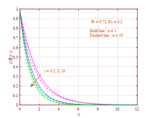
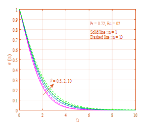
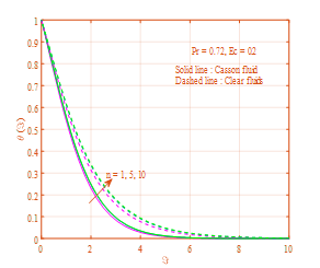
Figures 4 and 5 exhibit the distribution of non dimensional temperature for increasing values of β and n. In Figure 4 it is observed that as β raises the dimensionless temperature also raises. In other hand side it is noticed that for raising values of n a reverse trend exists for dimensionless temperature (see Figure 5). For distinct values of the viscous dissipation parameter Ec for linear and nonlinear stretching sheets the behavior of temperature profiles is demonstrate in Figure 6. With the increment of viscous dissipation parameter Ec the thickness of the boundary layer also increases as indicated in the figure. Here it is clear that the Ec number restricts the fluid motion and the value of Ec=0 represents no viscous dissipation. The reason behind is Eckert number Ec means it is the ratio of the square of velocity of fluid far-away from the surface of the boundary to the product of the fluid specific heat at constant temperature. In the case of viscous dissipation (Ec>0 or Ec<0), so that as the value of Ec the thermal boundary layer increases. The behavior of temperature profiles for distinct values of Prandtl number Pr for two linear and nonlinear stretching sheets can be found in Figure 7. It is notified from this figure that, the temperature profiles falls as the Prandtl number Pr rises, Moreover, the thermal boundary layer is thinner at large Pr. It is because of the small augment of the Prandtl number (Pr<<1).
Figure 4. Graph for SRM solutions of temperature for various values of β
Figure 5. Graph for SRM solutions of temperature for various values of n
Figure 6. Graph for SRM solutions of temperature for various values of Ec
Figure 7. Graph for SRM solutions of temperature for various values of Pr
A numerical study of free convection flow of Casson fluid in the presence of viscous dissipation over a non linear stretching sheet has been studied. In this study the effect of Casson parameter β, nonlinearity parameter n, viscous dissipation parameter Ec and Prandtl number Pr are discussed in detail and the outcomes are presented graphically along with tables. The observations of present study can be summarized as follows:
The outcomes may be useful for probable technological applications in liquid-based systems concerning elongated materials. Because of the numerical values are very close to exact values.
[1] Crane, L. (1970). Flow past a stretching plate. Journal of Applied Mathematics and Physics, 21: 645-647. https://doi.org/10.1007/BF01587695
[2] Sakiadis, B.C. (1961). Boundary layer behavior on continuous solid flat surfaces. American Institute of Chemical Engineers Journal, 7(1): 26-28. https://doi.org/10.1002/aic.690070108
[3] Tsou, F.K., Sparrow, E.M., Goldstein, R.J. (1967). Flow and heat transfer in the boundary layer on a continuous moving surface. International Journal of Heat and Mass Transfer, 10(2): 219-235. https://doi.org/10.1016/0017-9310(67)90100-7
[4] Noor, F.M, Kechil, S.A., Hashim, I. (2010). Simple nonperturbative solution for MHD viscous flow due to a shrinking sheet. Communications in Nonlinear Science and Numerical Simulation, 15(2): 144-148. https://doi.org/10.1016/j.cnsns.2009.03.034
[5] Prasannakumara, B.C., Ramesh, G.K., Gireesha, B.J. (2016). Melting and radiation effects on stagnation point Jeffrey fluid flow over a stretching sheet in the presence of nanoparticles. Journal of Nanofluids, 5(6): 993-999. https://doi.org/10.1166/jon.2016.1285
[6] Bilal, M., Hussain, S., Sagheer, M. (2017). Boundary layer flow of magneto-micropolar nanofluid flow with Hall and ion-slip effects using variable thermal diffusivity. Bulletin of the Polish Academy of Sciences: Technical Sciences, 65(3): 383-390. https://doi.org/10.1515/bpasts-2017-0043
[7] Mabood, F., Khan, W.A., Ismail, A.I.M. (2015). MHD boundary layer flow and heat transfer of nanofluids over a nonlinear stretching sheet: A numerical study. Journal of Magnetism and Magnetic Material, 374: 569-576. https://doi.org/10.1016/j.jmmm.2014.09.013
[8] Reher, E.O., Haroske, D., Kohler, K. (1969). Strömungen nicht-Newtonscher Flüssigkeiten. Chem. Technol., 21(3): 137-143.
[9] Walwander, W.P., Chen, T.Y, Cala, D.F. (1975). An approximate Casson fluid model for tube flow of blood. Biorheology, 12(2): 111-119. https://doi.org/10.3233/BIR-1975-12202
[10] Cokelet, G., Shin, H., Britten, A., Wells, R.E. (1963). Rheology of human blood - measurement near and at zero shear rate. Transactions of the Society of Rheology, 7(1): 303-317. https://doi.org/10.1122/1.548959
[11] Chevalley, J. (1991). An adaptation of the Casson equation for the rheology of chocolate. Journal of Texture Studies, 22(2): 219-229. https://doi.org/10.1111/j.1745-4603.1991.tb00015.x
[12] Garcia-Ochoa, F., Casas, J.A. (1994). Apparent yield stress in xanthan gum solutions at low concentrations. The Chemical Engineering Journal and the Biochemical Engineering Journal, 53(3): B41-B46. https://doi.org/10.1016/0923-0467(93)06043-P
[13] Kirsanov, E.A, Remizov, S.V. (1999). Application of the Casson model to thixotropic waxy crude oil. Rheologica Acta, 38: 172-176. https://doi.org/10.1007/s003970050166
[14] Joye, D.D. (1998). Application of yield stress-pseudoplastic fluid models to pipeline transport of sludge, in: Proc. 30th MidAtlantic Industrial Waste Conf. on Hazardous and Industrial Wastes, Technomic Publ. Corp., Lancaster, PA/Basel, pp. 567-575.
[15] Bird, R.B., Stewart, W.E., Lightfoot, E.N. (1960). Transport Phenomena. Wiley, New York. https://doi.org/10.1002/aic.690070245
[16] Wilkinson, W.L. (1960). Non-Newtonian Fluids. Pergamon, New York.
[17] Churchill, S.W. (1988). Viscous Flows- The Practical Use of Theory. Butterworths- Boston. Ch. 5. eBook.
[18] Boyd, J., Buick, J.M., Green, S. (2007). Analysis of the Casson and Carreau-Yasuda non-Newtonian blood models in steady and oscillatory flow using the lattice Boltzmann method. Physics of Fluids, 19(9): 93-103. https://doi.org/10.1063/1.2772250
[19] Nadeem, S., Haq, R.U., Lee, C. (2012). MHD fl ow of a Casson fluid over an exponentially shrinking sheet. Scientia Iranica. 19(6): 1550-1553. https://doi.org/10.1016/j.scient.2012.10.021
[20] Kumari, S., Murthy, M.V.R., Reddy, M.C.K., Kumar, Y.V.K.R. (2011). Peristaltic pumping of a magnetohydrodynamic Casson fluid in an inclined channel. Advance in Applies Science Research, 2(2): 428-436.
[21] Sreenadh, S., Pallavi, A.R., Satyanarayana, B. (2011). Flow of a Casson fluid through an inclined tube of non-uniform cross section with multiple stenoses. Advances in Applied Science Research, 2(5): 340-349.
[22] Mukhopadhyay, S., Ranjan De, P., Bhattacharyya, K., Layek, G.C. (2013). Casson fluid flow over an unsteady stretching surface. Ain Shams Engineering Journal, 4(4): 933-938. https://doi.org/10.1016/j.asej.2013.04.004
[23] Fung, Y.C. (1981). Biomechanics: Mechanical Properties of Living Tissues. Springer-Verlag, New York.
[24] Saqib, M., Ali, F., Khan, I. (2018). Heat and mass transfer phenomena in the flow of Casson fluid over an infinite oscillating plate in the presence of first-order chemical reaction and slip effect. Neural Computing & Applications, 30: 2159-2172. https://doi.org/10.1007/s00521-016-2810-x
[25] Vajravelu, K., Roper, T. (1999). Flow and heat transfer in a second grade fluid over a stretching sheet. International Journal of Non-linear Mechanic, 34(6): 1031-1036. https://doi.org/10.1016/S0020-7462(98)00073-0
[26] Alinejad, J., Samarbakhsh, S. (2012). Viscous flow over non-linearly stretching sheet with effects of viscous Dissipation. Jouranal of Applied Mechanics, 2012: 587834. http://dx.doi.org/10.1155/2012/587834
[27] Zaimi, K., Ishak, A., Pop, I. (2014). Flow past a permeable stretching/shrinking sheet in a nanofluid using two-phase model. Plos One, 9(11). https://doi.org/10.1371/journal.pone.0111743
[28] Dhanai, R., Rana, P., Kumar, L. (2016). MHD mixed convection nanofluid flow and heat transfer over an inclined cylinder due to velocity and thermal slip effects: Buongiorno’s model. Powder Technology, 288: 140-150. https://doi.org/10.1016/j.powtec.2015.11.004
[29] Goyal, M., Bhargava, R. (2014). Numerical study of thermo diffusion effects on boundary layer flow of nanofluids over a power law stretching sheet. Microfluidics and Nanofluidics, 17(3): 591-604. https://doi.org/10.1007/s10404-013-1326-2
[30] Shen, M., Wang, F., Chen, H. (2015). MHD mixed convection slip flow near a stagnation-point on a non-linearly stretching sheet. Boundary Value Problems, 78: 1-15. https://doi.org/10.1186/s13661-015-0340-6
[31] Jat, R.N., Chaudhary, S., Angew, Z. (2010). Radiation effects on the MHD flow near stagnation-point of a stretching sheet. Zeitschrift für angewandte Mathematik und Physik, 61: 1151-1154. https://doi.org/10.1007/s00033-010-0072-5
[32] Dessie, H., Kishan, N. (2014). HMD effects on heat transfer over stretching embedded in porous medium with variable viscosity Viscous dissipation and heat source/sink. Engineering Physics and Mathematics, Ain Shams Engineering Journal, 5(3): 967-977. https://doi.org/10.1016/j.asej.2014.03.008
[33] Mukhopadhyay, S. (2013). Casson fluid flow and heat transfer over a nonlinearly stretching surfac. Chinese Physics B, 22(7).
[34] Motsa, S.S. (2014). A new spectral relaxation method for similarity variable nonlinear boundary layer flow systems. Chemical Engineering Communications. 201(2): 241-256. https://doi.org/10.1080/00986445.2013.766882
[35] Canuto, C., Hussaini, M.Y., Quarteroni, A.M., Zang, T.A. (1988). Spectral Methods in Fluid Dynamics. Springer, Berlin. https://doi.org/10.1007/978-3-642-84108-8
[36] Trefethen, L.N. (2000). Spectral Methods in MATLAB. SIAM, Philadelphia. http://dl.merc.ac.ir/handle/Hannan/7375.
[37] Rana, P., Bhargava, R. (2012). Flow and heat transfer of a nanofluid over a nonlinearly stretching sheet a numerical study. Communications in Nonlinear Science and Numerical Simulation, 17(1): 212-226. https://doi.org/10.1016/j.cnsns.2011.05.009
[38] Cortell, R. (2007). Viscous flow and heat transfer over a nonlinearly stretching sheet. Applied Mathematics and Computation, 184(2): 864-873. https://doi.org/10.1016/j.amc.2006.06.077
[39] Zaimi, K., Ishak, A., Pop, I. (2014). Boundary layer flow and heat transfer over a nonlinearly permeable stretching/shrinking sheet in a nanofluid. Scientific Reports, 4: 4404. http://dx.doi.org/10.1038/srep04404
[40] Khan, W.A., Pop, I. (2010). Boundary layer flow of a nanofluid past a stretching sheet. International Journal of Heat and Mass Transfer, 53(11-12): 2477-2483. https://doi.org/10.1016/j.ijheatmasstransfer.2010.01.032
[41] Wang, C.Y. (1989). Free convection on avertical stretching surface. Journal of Applied Mathematics and Mechanics, 69(11): 418-420. https://doi.org/10.1002/zamm.19890691115
[42] Gorla, R.S.R., Sidawi, I. (1994). Free convection on a vertical stretching surface with suction and blowing. Applied Scientific Research, 52: 247-257. https://doi.org/10.1007/BF00853952