Munagala Venkata Subba Rao* | Kotha Gangadhar| Giulio Lorenzini
OPEN ACCESS
The present paper intends to investigate and highlight the steady, two dimensional flow of heat and mass transfer of magneto hydrodynamic tangent hyperbolic fluid with suction/injection. In the present study tangent hyperbolic fluid is considered as the working fluid to investigate. The obvious viscosity of the study is varies to the extreme points i.e. between zero shear rates to the shear rate of infinity. Due to the stretching flow is induced. To get the numerical solution the powerful numerical technique that is spectral relaxation method is applied for the set of transformed equations those are derived from physical model of the flow. Thereafter, numerical outcomes are computed to discuss the convergence and accuracy of the proposed technique. The impacts of different flow controlling parameters which are experienced in the problem are resolved. All the obtained outcomes from the above numerical procedure are displayed through graphs and tables to discuss various resulting parameters. The main notable observations are it is found that on increasing Power law index (n) causes considerable increase in the thickness of the fluid. Therefore, the velocity profiles are decreased. Further, on increasing power law index causes considerable increase in both thicknesses of thermal and concentration boundary layers.
stretching sheet, tangent hyperbolic fluid, suction/injection, SRM
In recent years studies about the flows of boundary layer of non-Newtonian model liquids on extending sheet have been inspected for a long time on account of their tremendous applications in various assembling procedure, for example, in polymer, material, sustenance preparing businesses and so forth. In current time enterprises the uses of non-Newtonian liquids exceed expectations that of Newtonian one. The usage of such liquids can be supported by utilizing a few added substances. In any assembling procedure the magnificence of the final results of such enterprises estimated based on the cooling rate in heat exchange methods because it decides the quality of desired characteristics of the final product. The magneto hydrodynamic is one of the factors by which the cooling rate can be distributed and the happen to the favoured component can achieved. Considered tangent hyperbolic fluid is a working fluid in the present study which is also a non-Newtonian fluid model. The tangent hyperbolic fluid is used extensively for different research facility tests. Then again, because of the considerable applications in polymer preparing enterprises, the researchers have demonstrated their enthusiasm to ponder the time- independent flow of non-Newtonian fluids by means of a clear yield value through tubes. Wang [1] studied about the flow of the fluid at outside of stretching cylinder. Afterward, Majeed et al. [2] analyzed about heat transfer analysis over a hyperbolic stretching cylinder. Furthermore, by means of numerical strategy Mukhopadhyay [3] analyzed the heat transfer along with boundary layer flow in a porous medium over a stretching cylinder.
Afterward, Wang [4] analyzed very strategically about mixed convection heat transfer analysis in between non-Newtonian fluid model and vertical plate by introducing mixed convection parameter by means of unvarying heat of the wall. Further, a detailed notable effect of the laminar mixed convection flow of non-Newtonian was investigated by Hady [5]. Later, Gorla [6] presented a detail discussion about the buoyancy force how it effects the friction factor, the non dimensional rate of heat transfer and also about the details of velocity, temperature fields by means of numerical method. Furthermore, by means of numerical technique i.e., fourth order of R-K method together with shooting scheme, Mostafa [7] noted that there is a corresponding decrease in coefficient of skin friction together with slip parameter increments. Later on Mehdy [8] obtained the numerical solutions of flow and heat transfer for non-Newtonian fluid outside a stretching cylinder by means of various parameters, moreover the behaviour of non-Newtonian fluid is characterised by means of Casson fluid model. Further, Ghaffari et al. [9] presented the non-linear radiation effect in non-Newtonian fluid in a permeable media with stagnated point flow. Furthermore, Chen and Leonard [10] observed that transverse curvature shows a significant impact on skin friction from the leading edge with the help of series solution.
Moreover, Pop et al. [11] they explained about the how the profiles of velocity and temperature are persuade based on the sort of power-law of the fluid, parameter of the curvature and Prandtl number considerably likewise heat transfer coefficient. Further, Nadeem and Akram [12] in their study they observed that large pressure attention of gradient is very essential for studying channel narrow part moreover pressure gradient is decreased along with weissenberg number and width of the channel increments. Afterward, in one more production they [13] clarified obviously about the partial slip effects in peristaltic transport of a hyperbolic tangent fluid. Later, Naseer et al. [14] in their work they examined by means of numerical strategy about boundary layer flow and heat exchange in a working fluid that is tangent hyperbolic fluid in the direction of axial over a vertical exponentially stretching.
Many researchers are showing their enthusiasm to study the MHD flow due to the notable applications in engineering see for example, in pumps, meters, generators and bearings. Effect of MHD and heat transfer consequences for a flow of boundary layer of power law non-Newtonian over a vertical stretching sheet is considered by Ferdows and Hamad [15]. Later, Satyanarayana and Harish Babu [16] considered Jeffrey fluid which is electrically conducted in his study to examine the effects of chemical reaction and radiation of heat on magneto hydrodynamics heat and mass transmit over a stretchable sheet. In addition, Ashorynejad et al. [17] called attention to the eminent comments about the effects of volume fraction of nanoparticle, sort of nanofluid, parameter of magnetic and Reynolds number on the flow and heat exchange characteristics by means of numerical strategy. Afterward, Kandaswamy et al. [18] deliberated about a mixed convection flow of transfer of heat and mass with the effect of magneto hydrodynamics over a permeable medium.
In addition, Kumari and Nath [19] in their work they mainly concluded that there is a significant improvement in coefficient of heat exchange with the Prandtl number. Moreover velocity gradient is negative if wall velocity is more noteworthy than that of free stream velocity while velocity gradient is positive if wall velocity is not as much as free stream velocity. Later, Seth et al. [20] presented a hypothetical investigation and noted some of the significant outcomes of the study and in course of time, observed that there is a decrement in case of primary skin friction while there exist a increment in case of secondary skin friction, this observation is one of the outcome in their study. Further, Awais et al. [21] has been analysed noticeably about the impacts of momentum and heat transfer analysis of Sisko fluid near the axisymmetric near to the stagnation point in the direction of a stretching cylinder. Recently, Gangadhar et al. [22] considered numerical study on the viscous dissipation and variable suction/injection on boundary layer flow. They [23] further explored some features about the unsteady boundary layer flow of nanofluid with the assistance of the numerical strategy that is spectral relaxation scheme. In another work he [24] presented the features of MHD micropolar nanofluid by considering Newtonian heating. Further, Venkata Subba Rao et al. [25] considered numerical study on analysis of heat transfer on Casson fluid in presence of thermal radiation and applied transverse magnetic field with the help of powerful assistance of the numerical strategy that is spectral relaxation scheme. Later, in another work they [26] have studied numerically about the features of magneto hydrodynamic boundary layer flow of nanofluid. Ibrahim [27] analyzed very clearly about the impact of thermal radiation on MHD flow of tangent hyperbolic fluid which is a non- Newtonian medal by means of nanoparticle past an stretchable sheet by means of slip with order two as well as convective boundary condition. Later, Mahdi Ramezanizadeh et al. [28] they concluded that thermosyphons are utilized in different energy systems because of their substantial performance in heat transfer. There are many substantial practical applications in science and engineering by studying the tangent hyperbolic fluid as working fluid.
The specific objective of current analysis is to explore the heat and mass transfer of magneto hydrodynamics tangent hyperbolic fluid by considering the magnetic field with the help of proposed convergent numerical technique SRM and how the various physical parameters all those are involved in the problem are effect the fluid flow and those effects are examined through graphs and table. Also all the obtained outcomes are shows correlation among the available results in literature.
To analyze the present problem in detail let us take steady, incompressible, 2D flow of electrically conducting (σ) tangent hyperbolic fluid past a stretching cylinder. Because of the stretching there exist a velocity that is denoted with $U_w (x)$ and it is defined as $U_w (x)=ax/l$, here a is called positive constant and l is called characteristic length. Fluid is filled at the upper half of the plate that is r>R. Due to the stretching flow is induced. The constitutive equation of tangent hyperbolic fluid, (See, Akbar et al. [29]) is given by
$\bar{\tau }=\left[ {{\mu }_{\infty }}+({{\mu }_{0}}+{{\mu }_{\infty }})\tanh {{\left( \Gamma \bar{\dot{\gamma }} \right)}^{n}} \right]\bar{\dot{\gamma }}$ (1)
The flow behaviour index is denoted with $\bar{\dot{\gamma }}$, it is given by
$\bar{\dot{\gamma }}=\sqrt{\frac{1}{2}\sum\limits_{i}{\sum\limits_{j}{{{{\bar{\dot{\gamma }}}}_{ij}}{{{\bar{\dot{\gamma }}}}_{ji}}}}}=\sqrt{\frac{1}{2}\Pi }$ (2)
Here, $Π=1/2 tr(gradV+(gradV)^T )^2$. If μ_∞=0 in Equation (1) then it is unrealistic to examine the issue of the infinite shear rate viscosity, moreover the considered working fluid has the shear thinning impacts, so that $Γ\bar{\dot{\gamma }}<1$, because of this equation (1) is expressed as follow:
$\begin{align} & \bar{\tau }={{\mu }_{0}}\left[ {{\left( \Gamma \bar{\dot{\gamma }} \right)}^{n}} \right]\bar{\dot{\gamma }}={{\mu }_{0}}\left[ {{\left( 1+\Gamma \bar{\dot{\gamma }}-1 \right)}^{n}} \right]\bar{\dot{\gamma }} \\ & \,\,\,\,={{\mu }_{0}}\left[ \left( 1+n(\Gamma \bar{\dot{\gamma }}-1) \right) \right]\bar{\dot{\gamma }} \\\end{align}$ (3)
The external force f is formulated below:
$f=J\times B$ (4)
Here, current density is with J and it defined as $J=σ_0 (E+V×B)$ and $B=(0,B_0)$ is the applied magnetic field with transverse uniform time dependent to the fluid layer. The electric field and electric conductivity are represented with the symbols E and σ0 respectively. It is assumed that external electric field does not exist. With this assumption the induced magnetic field and the magnetic Reynolds number become considerably negligible. Consequently, the Hall Effect is not in consideration. Figure 1 represents the coordinate system as well as physical model of the considered problem.

Figure 1. Physical model of the considered problem
By means of above supposing assumptions governing equations for the flow of present considered model are:
$\frac{\partial (ru)}{\partial x}+\frac{\partial (rv)}{\partial r}=0$ (5)
$\begin{align} & u\frac{\partial u}{\partial x}+v\frac{\partial u}{\partial r}=\upsilon (1-n)\frac{{{\partial }^{2}}u}{\partial {{r}^{2}}}+(1-n)\frac{1}{r}\frac{\partial u}{\partial r} \\ & +\sqrt{2}n\Gamma \left( \frac{\partial u}{\partial r} \right)\frac{{{\partial }^{2}}u}{\partial {{r}^{2}}}+\frac{n\Gamma }{\sqrt{2}r}{{\left( \frac{\partial u}{\partial r} \right)}^{2}}-\frac{\sigma B_{0}^{2}}{\rho }u \\\end{align}$ (6)
$u\frac{\partial T}{\partial x}+v\frac{\partial T}{\partial r}=\alpha \left( \frac{1}{r}\frac{\partial T}{\partial r}+\frac{{{\partial }^{2}}T}{\partial {{r}^{2}}} \right)$ (7)
$u\frac{\partial C}{\partial x}+v\frac{\partial C}{\partial r}=\alpha \left( \frac{1}{r}\frac{\partial C}{\partial r}+\frac{{{\partial }^{2}}C}{\partial {{r}^{2}}} \right)$ (8)
The following are considered as boundary conditions:
$r=R:u={{U}_{w}}(x)=\frac{ax}{l},v={{v}_{0}},T={{T}_{w}},C={{C}_{w}}$ (9)
$r\to \infty :u\to {{U}_{\infty }}(x)=0,T\to {{T}_{\infty }},C\to {{C}_{\infty }}$ (10)
Here, similarity transformations can be chosen for finding the similarity solution and they are as follow:
$\begin{align} & u=\frac{1}{r}\frac{\partial \psi }{\partial r},v=-\frac{1}{r}\frac{\partial \psi }{\partial x}, \\ & \eta =\sqrt{\frac{a}{l\upsilon }}\left( \frac{{{r}^{2}}-{{R}^{2}}}{2R} \right),\,\,\psi =\sqrt{\frac{\upsilon ax}{l}}Rf\left( \eta \right), \\ & \theta (\eta )=\frac{T-{{T}_{\infty }}}{{{T}_{w}}-{{T}_{\infty }}},\varphi (\eta )=\frac{C-{{C}_{\infty }}}{{{C}_{w}}-{{C}_{\infty }}} \\\end{align}$ (11)
Making use of transformations (11), equations (5)-(10) can be written as:
$\begin{align} & (1-n)(1+2K\eta ){{{f}'}'}'+f{{f}'}'-{{{{f}'}}^{2}}+2K(1-n){{f}'}' \\ & +2\lambda n{{(1+2K\eta )}^{3/2}}{{f}'}'{{{f}'}'}' \\ & +3\lambda K{{(1+2K\eta )}^{1/2}}{{{{{f}'}'}}^{2}}-M{f}'=0 \\\end{align}$ (12)
$(1+2K\eta ){{\theta }'}'+2K{\theta }'+\Pr f{\theta }'=0$ (13)
$(1+2K\eta ){{\varphi }'}'+2K{\varphi }'+Scf{\varphi }'=0$ (14)
Boundary conditions after transformation as follow:
$f(0)={{f}_{w}},{f}'(0)=1,\theta (0)=1,\varphi (0)=1$ (15)
${f}'(\infty )=0,\theta (\infty )=0,\varphi (\infty )=0$ (16)
Non dimensional constants which are involved in equations (12)-(14) are the Weissenberg number λ, suction/injection parameter fw Prandtl number is denoted with Pr, magnetic parameter is denoted with , curvature parameter is denoted with K and the Schmidt number is denoted with Sc and all these are formulated as follow:
$\begin{align} & \lambda =\frac{\sqrt{a}\Gamma {{U}_{w}}}{\sqrt{2l\upsilon }},{{f}_{w}}=-\frac{{{v}_{0}}r}{R}\sqrt{\frac{l}{\upsilon a}},\Pr =\frac{\upsilon }{\alpha }, \\ & M=\frac{\sigma B_{0}^{2}l}{\rho a},K=\left( \frac{1}{R} \right)\sqrt{\frac{\upsilon l}{a}},Sc=\frac{\alpha }{D} \\\end{align}$ (17)
The wall shearing stress $τ_w$ at the surface is defined as
${{\tau }_{w}}=\mu {{\left[ (1-n)\frac{\partial u}{\partial r}+\frac{n\Gamma }{\sqrt{2}}{{\left( \frac{\partial u}{\partial r} \right)}^{2}} \right]}_{r=R}}$ (18)
Here μ is the viscosity coefficient.
The coefficient of skin friction can be written as:
${{C}_{f}}=\frac{{{\tau }_{w}}}{\rho U_{w}^{2}}$ (19)
From the equations (17) and (18), the formula for the coefficient of skin friction is as follow:
${{C}_{fx}}\operatorname{Re}_{x}^{1/2}=\left[ (1-n){f}''(0)+n\lambda {{\left( {f}''(0) \right)}^{2}} \right]$ (20)
At the wall surface heat flux can be written as follow:
${{q}_{w}}=-k{{\left( \frac{\partial T}{\partial r} \right)}_{r=R}}$ (21)
The formula for Nusselt number is as follow:
$N{{u}_{x}}=\frac{x}{k}\frac{{{q}_{w}}}{{{T}_{w}}-{{T}_{\infty }}}$ (22)
At the wall heat transfer rates with the help of Equations (21) and (22) is as follow:
$\frac{N{{u}_{x}}}{\operatorname{Re}_{x}^{1/2}}=-{\theta }'(0)$ (23)
Formula for mass flux at surface is as follow:
${{J}_{w}}=-D{{\left( \frac{\partial C}{\partial r} \right)}_{r=R}}$ (24)
The Sherwood ($Sh_x$) is given by
$S{{h}_{x}}=\frac{x}{D}\frac{{{J}_{w}}}{{{C}_{w}}-{{C}_{\infty }}}$ (25)
By means of equations (24) in (25), the non-dimensional rate of wall mass transfer is given by
$\frac{S{{h}_{x}}}{\operatorname{Re}_{x}^{1/2}}=-{\varphi }'(0)$ (26)
In equations (20), (23) and (26), the local Reynolds number is denoted with $Re_x$ and it can be defined as:
${{\operatorname{Re}}_{x}}=\frac{x{{U}_{w}}(x)}{\upsilon }$
SRM is in use to solve equations (12)-(14) along with appropriate boundary conditions (15)-(16); it is proposed by Motsa et al. [30] and Kameswaran et al. [31]. The algorithm Spectral Relaxation Method is used to obtain the solution of similarity boundary layer problems with exponentially decay profiles. With the help of Chebyshev spectral collocation methods differential equations are discretized in this study (see for example Canuto [32] and Trefethen [33]). To get the ample accuracy of SRM we consider the number of grid points are 100 all the way through numerical experimentation is that $η_∞=15$. With regards to the spectral relaxation method iteration scheme depicted above, equations (12)-(16) become
${{{f}'}_{r+1}}={{p}_{r}},{{f}_{r+1}}(0)={{f}_{w}}$ (27)
$\begin{align} & (1-n)(1+2K\eta ){{{{p}''}}_{r+1}}+{{f}_{r+1}}{{{{p}'}}_{r+1}}+2\lambda (1-n){{{{p}'}}_{r+1}} \\ & +2\lambda n{{\left( 1+2K\eta \right)}^{3/2}}{{{{p}'}}_{r+1}}{{{{{p}'}'}}_{r+1}} \\ & +3\lambda K{{(1+2K\eta )}^{1/2}}{{{{p}'}}_{r+1}}^{2}-M{{p}_{r+1}}=p_{r}^{2} \\\end{align}$ (28)
${{{\theta }''}_{r+1}}(1+2K\eta )+2K{{{\theta }'}_{r+1}}+\Pr {{f}_{r+1}}{{{\theta }'}_{r+1}}=0$ (29)
${{{{\varphi }'}'}_{r+1}}(1+2K\eta )+2K{{{\varphi }'}_{r+1}}+Sc\left( {{f}_{r+1}} \right){{{\varphi }'}_{r+1}}=0$ (30)
By the iteration scheme the boundary conditions changes as
${{p}_{r+1}}(0)=1,{{\theta }_{r+1}}(0)=1,{{\varphi }_{r+1}}(0)=1$ (31)
${{p}_{r+1}}(\infty )=0,{{\theta }_{r+1}}(\infty )=0,{{\varphi }_{r+1}}(\infty )=0$ (32)
With a particular goal to be got finally, we apply the Chebyshev spectral collocation technique to decipher or make clear the decoupled equations (27)-(30). In the process of spectral relaxation method, the computational space of the domain [0, L] is changed to the interval [-1, 1] in Chebyshev spectral collocation method utilizingη=L(ξ+1)/2 on which the spectral technique is actualized. Here, L invokes the infinity boundary conditions. In spectral method the purpose of introducing D, where D is the differentiation matrix, is to estimate the unknown variables and its derivatives at the collocation points. The following representation is the matrix vector product
$\frac{\partial {{f}_{r+1}}}{\partial \eta }=\sum\limits_{k=0}^{{\bar{N}}}{{{D}_{lk}}{{f}_{r}}({{\xi }_{k}})}=D{{f}_{r}},l=0,1,2,.\cdots \cdots \cdots \bar{N}$ (33)
Here D = 2D/L and the vector function $f=[f(ξ_0),f(ξ_1),.........f(ξ_N ̄ )]^T$ is defined at grid points.
The powers of D denote the higher-order derivatives, i.e.
${{f}_{r}}^{(p)}={{D}^{p}}{{f}_{r}}$ (34)
The order of the derivative is denoted by p. Applying the proposed technique to equations (27)-(30), we get,
${{A}_{1}}{{f}_{r+1}}={{B}_{1}},{{f}_{r+1}}({{\xi }_{{\bar{N}}}})={{f}_{w}}$ (35)
${{A}_{2}}{{p}_{r+1}}={{B}_{2}},{{p}_{r+1}}({{\xi }_{{\bar{N}}}})=1,{{p}_{r+1}}({{\xi }_{0}})=0$ (36)
${{A}_{3}}{{\theta }_{r+1}}={{B}_{3}},{{\theta }_{r+1}}({{\xi }_{{\bar{N}}}})=1,{{\theta }_{r+1}}({{\xi }_{0}})=0$ (37)
${{A}_{4}}{{\varphi }_{r+1}}={{B}_{4}},{{\varphi }_{r+1}}({{\xi }_{{\bar{N}}}})=1,{{\varphi }_{r+1}}({{\xi }_{0}})=0$ (38)
Here,
${{A}_{1}}=D,{{B}_{1}}={{p}_{r}}$ (39)
$\begin{align} & {{A}_{2}}={{D}^{2}}diag((1-n)(1+2K\eta ) \\ & +2\lambda n{{(1+2K\eta )}^{3/2}}{{{{p}'}}_{r+1}}) \\ & +diag\left( {{f}_{r+1}}+2K(1-n) \right)D-MI,{{B}_{2}}=p_{r}^{2} \\\end{align}$ (40)
$\begin{align} & {{A}_{3}}=diag(1+2K\eta ){{D}^{2}}+diag\left( \Pr {{f}_{r+1}}+2K \right)D \\ & -diag(\Pr \eta {{p}_{r+1}})I,{{B}_{3}}=0 \\\end{align}$ (41)
$\begin{align} & {{A}_{4}}=diag(1+2K\eta ){{D}^{2}}+diag\left( Sc{{f}_{r+1}}+2K \right)D \\ & -diag(Sc\eta {{p}_{r+1}})I,{{B}_{4}}=0 \\\end{align}$ (42)
In equations (39)-(42), an identity matrix represented by I, and diagonal matrix represented by diag[], at the grid points the values of the functions f, p, θ and φ are f, p, θ and φ respectively, where the subscript r represents an iteration number.
To start the SRM scheme for equations (27)-(32) the initial guesses are chosen as follow:
$\begin{align} & {{f}_{0}}(\eta )={{f}_{w}}+1-{{e}^{-\eta }},p{}_{0}\left( \eta \right)={{e}^{-\eta }}, \\ & {{\theta }_{0}}\left( \eta \right)={{e}^{-\eta }},{{\varphi }_{0}}\left( \eta \right)={{e}^{-\eta }} \\\end{align}$ (43)
All the functions are chosen randomly and all these functions are satisfying the boundary conditions. The purpose of repeating the iteration scheme is to get the convergence. In terms of infinity norm of spectral relaxation method the convergence is explained by
$Er=Max\left( \begin{align} & \left\| {{f}_{r+1}}-{{f}_{r}} \right\|,\left\| {{p}_{r+1}}-{{p}_{r}} \right\|, \\ & \left\| {{\theta }_{r+1}}-{{\theta }_{r}} \right\|,\left\| {{\varphi }_{r+1}}-{{\varphi }_{r}} \right\| \\\end{align} \right)$ (44)
The main purpose of increasing the number of grid points to build up the exactness of the proposed scheme, moreover to obtain consistent solutions for any further increments also.
Numerical computations are shown graphically in Figure 2 to Figure 15 to discuss various resulting parameters which are involved the problem. The outcomes which are obtained from the numerical procedure discussed in the previous section are compared with those of Akber et al. [29] and Malik et al. [34] and displayed in Table 1. This comparison shows a decent agreement between present study and previous studies. Furthermore, the outcomes demonstrate that the spectral relaxation method is efficient and adequately powerful for use of solving fluid flow problems.
Table 1. Comparison of coefficient of Skin friction $\sqrt{{{\operatorname{Re}}_{x}}}{{C}_{fx}}$ with the available results in literature for various values of M when Pr=Sc=n=K=λ=0
|
$\sqrt{{{\operatorname{Re}}_{x}}}{{C}_{fx}}$ |
|||
|
|
Present Study (SRM) |
Akbar (Runge–Kutta–Fehlberg method) [29] |
Malik (Kellor-Box method) [34] |
|
0 0.5 1 5 10 100 500 1000 |
1 -1.118034 -1.414214 -2.449490 -3.316625 -10.049874 -22.383029 -31.638584 |
1 -1.11803 -1.41421 -2.44949 -3.31663 -10.04988 -22.38303 -31.63859 |
1 -1.11802 -1.41419 -2.44945 -3.31657 -10.04981 -22.38294 -31.63851 |
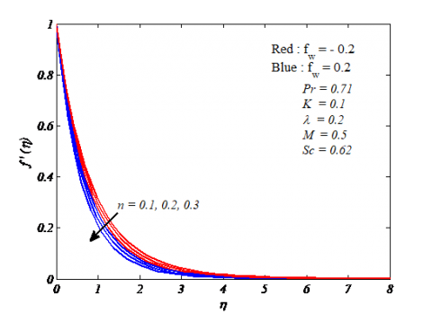
Figure 2. Variation of velocity profile $f'(η)$ for
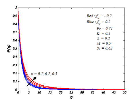
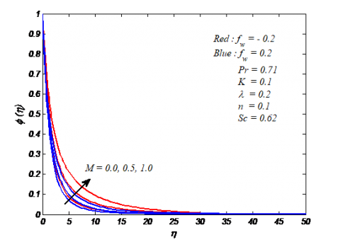
Particularly, Figures 2-12 show the characteristics of emerging parameters those are involved in the problem. The Figures 2-4 describe the distribution of velocity, temperature mass friction function for the varying values of power law index for both cases i.e., suction and injection here suction is with $f_w>0$ and injection is denoted with $f_w<0$. In this regard, it can be noticed from Figure 2, that velocity profiles decreased for rising values of n. It is because of increments in n there is an increase in the thickness of the fluid. From the Figures 3 and 4, it tends to be seen that increment in the profiles of temperature and concentration by increasing n and also it tends to be seen that, thermal and concentration boundary layer thickness increased. Moreover, from the same figures it tends to be found that, velocity, temperature and concentration decreased for suction or injection parameter increments. The distribution of velocity, temperature and concentration for both suction and injection due to the applied magnetic parameter M in order is shown Figures 5, 6 and 7.
Figure 3. Variation of temperature profile θ(η) for n
Figure 4. Variation of concentration profile φ(η) for n
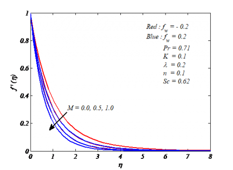
Figure 5. Variation of velocity profileb $f'(η)$ for M
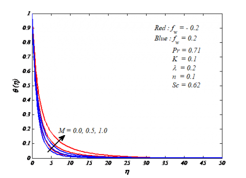
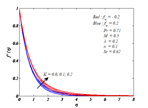
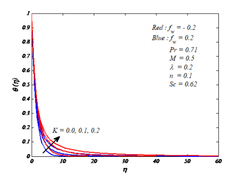
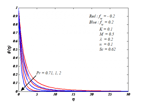
From Figure 5, noticed that velocity profile is diminished along with the increase of M; it is because of increment in the magnetic field strength. For M = 0, indicates flow is hydrodynamic while for M ≠ 0 indicates the flow is magnetic flow case. The reason for the decrease in velocities is that magnetic field is always normal to an electrically conducting fluid flow, so that there is a resistive force to the flow. This opposing force is named as Lorentz force. As a result, there exists a retardation effect on the fluid flow. Due to this there exists a deceleration in the velocity. Moreover, increase in its boundary layer thickness is observed. It tends to be seen that, temperature, concentration profiles and also corresponding boundary layer thickness is significantly increased along with the increase in M, this can be shown in Figures 6 and 7. We can observe that enhancement in the fluid velocity profiles along with the rising of curvature parameter K as shown in Figure 8. The reason is that with the increasing values of K there exist a reduction in the curvature radius the reason behind is that area of the cylinder reduces. Because of this reason fluid particle gets a low resistive force to the cylinder. With this velocity of the fluid enhances. Also Figures 9 and 10 portrays profiles of temperature and concentration respectively under the influence of K. Moreover, we can notice from the same figures, that curvature parameter K enhances the fluid temperature, concentration and also boundary layers of thermal and concentration respectively. The reason is that parameter of curvature K accelerates the rates of heat and mass transmits significantly as a result we can notice an upsurge in the fluid temperature and concentration. In general, the relation between fluid kinematic viscosity and thermal diffusivity is named as the Prandtl number. From the Figure 11, noticed that temperature and corresponding thickness of the thermal boundary layer are decreased for Prandtl number increments. Reason behind this is that, increase in Pr means increases in viscosity of the fluid and rate of heat transfers increase. It is the reason for decrement in the fluid temperature.
Figure 6. Variation of temperature profile θ(η) for M
Figure 7. Variation of concentration profile φ(η) for M
Figure 8. Variation of velocity profile f^' (η) for K
Figure 9. Variation of temperature profile θ(η) for K
Figure 10. Variation of concentration profile φ(η) for K
Figure 11. Variation of temperature profile θ(η) for Pr
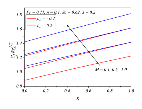
Figure 12 is drawn to demonstrate the concentration profile for varying values of Schmidt number Sc. The values for Sc are selected as 0.24, 0.62 and 0.78 to signifying the diffusing chemical species in gasses like $H_2$, $H_2 O$ and $NH_3$ respectively. From Figure 12, it tends to be seen that, fluid concentration decreased with the increase of Sc. Figure 13 is used to understand the behaviour of skin friction for various resulting parameters which are encountered in the present problem. From this plot noticed that skin friction coefficient is increased along with the rise of flow controlling parameters like, magnetic, curvature and suction/injection.
Figure 12. Variation of concentration profile φ(η) for Sc
Figure 13. Variation of skin friction coefficient $C_f Re_x^{1/2}$ for M&K
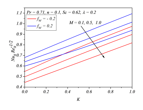
Figure 14. Variation of local Nusselt number $Nu_xRe_x^{-1/2} for M&K
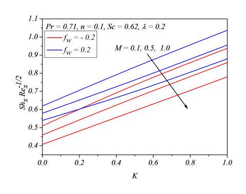
Figure 14 represents the performance of local Nusselt number on fluid for various resulting parameters. It tends to be observing there exist an increase in local Nusselt number with the rising of parameters of curvature K and suction/injection Fw while opposite results are obtained for magnetic field strength. Figure 15 presents the behaviour of local Sherwood number for different fluid parameters. From this figure it tends to be found that increase in curvature parameter K and suction/injection parameter Fw causes corresponding increase in local Sherwood number while opposite results are obtained for magnetic field strength.
Figure 15. Variation of Sherwood number $Sh_xRe_x^{-1/2}$ for M&K
From the present analysis is laid out to analyse the transfer of heat and mass in magneto hydrodynamics tangent hyperbolic fluid flow past a stretchable cylinder by means of thermal dispersion and suction/injection by means of proposed numerical technique. A set of transformed equations which are obtained from the governing partial differential equations are solved numerically with the help of convergent numerical technique that is Spectral Relaxation Method. The numerical solutions are displayed through graphs and tables and found a decent agreement with the previously presented outcomes in the literature. From above analysis some of the main observations are summarizes as follow:
$k$ Thermal conductivity of the fluid (W/m K)
${{c}_{p}}$ Specific heat maintained at unvarying pressure (J/kg K)
$f$ Non dimensional stream function
$u,v$ Velocity components (m/s)
$x,r$ Dimensionless coordinates
$\gamma $ Mechanical thermal dispersion coefficient
$T$ Temperature fluid (0C)
${{T}_{w}}$ Surface temperature
${{T}_{\infty }}$ Fluid ambient temperature
${{u}_{w}}(x)$ Stretching velocity
$i$ Time index at the time of navigation
$L$ Scale
$t$ Time
$\overline{N}$ Number of grid points
${{C}_{fx}}$ Coefficient of skin friction
$C$ Fluid concentration
$C{}_{\infty }$ Fluid ambient concentration
${{C}_{w}}$ Concentration at the stretching surface
Greek symbols
$\alpha $ Fluid thermal diffusivity (m2/s)
$\mu $ Fluid thermal viscosity (N s/m)
$\rho $ Density (kg/m3)
${{\tau }_{w}}$ At wall shear stress
$\varphi $ Non-dimensional concentration
$\eta $ Similarity variable
$\upsilon =\frac{\mu }{\rho }$ Kinematic viscosity of the fluid
${{\mu }_{o}}$ Zero shear rate of viscosity of the fluid
${{\mu }_{\infty }}$ Infinite shear rate of viscosity of the fluid
$\Gamma $ Material constant with time dependent
$\theta $ Dimensionless temperature
Subscript
$w$ Surface condition
$\infty $ Infinity condition
Super script
' Derivative with respect to $\eta $
[1] Wang CY. (1988). Fluid flow due to a stretching cylinder. Phys Fluids 31: 466-468. https://doi.org/10.1063/1.866827
[2] Majeed A, Javed T, Mustafa I. (2016). Heat transfer analysis of boundary layer flow over hyperbolic stretching cylinder. Alexandria Eng J. 55: 1333-1339. https://doi.org/10.1016/j.aej.2016.04.028
[3] Mukhopadhyay S. (2012). Analysis of boundary layer flow and heat transfer along a stretching cylinder in a porous medium. ISRN Thermo Dynamics. http://dx.doi.org/10.5402/2012/704984
[4] Wang TY. (1995). Mixed convection from a vertical plate to non-Newtonian fluids with uniform surface heat flux. Int Commun Heat Mass J. 22(3): 369-380. https://doi.org/10.1016/0735-1933(95)00017-S
[5] Hady FM. (1995). Mixed convection boundary-layer flow of non-Newtonian fluids on a horizontal plate. Appl. Math. Comput. 68: 105-112. https://doi.org/10.1016/0096-3003(94)00084-H
[6] Gorla RSR. (1986). Combined forced and free convection in boundary layer flow of non-Newtonian fluid on a horizontal plate. Chem Eng Commun. 49: 13-22. https://doi.org/10.1080/00986448608911790
[7] Mostafa AAM. (2011). Slip velocity effect on a non-Newtonian power-law fluid over a moving permeable surface with heat generation. Math Comput Model. 54: 1228-1237. https://doi.org/10.1016/j.mcm.2011.03.034
[8] Mahdy A. (2015). Heat transfer and flow of a Casson fluid due to a stretching cylinder with the Soret and Dufour effects. J Eng Phys Thermo phys. 88(4): 928-936. https://doi.org/10.1007/s10891-015-1267-6
[9] Ghaffari A, Jayed T, Majeed A. (2016). Influence of radiation on non-newtonian fluid in the region of oblique stagnation point flow in a porous medium: A numerical study. Transport Porous Med. 113(1): 245-266. https://doi.org/10.1007/s11242-016-0691-1
[10] Chen SS, Leonard R. (1972). The axisymmetrical boundary layer for a power-law non-Newtonian fluid on a slender cylinder. Chem Eng J. 3: 88-92. https://doi.org/10.1016/0300-9467(72)85009-3
[11] Pop I, Kumari M, Nath G. (1990). Non-Newtonian boundary layers on a moving cylinder. Int J Eng Sci. 28(4): 303-312. https://doi.org/10.1016/0020-7225(90)90103-P
[12] Nadeem S, Akram S. (2009). Peristaltic transport of a hyperbolic tangent fluid model in an asymmetric channel. Zeitschriftfür Naturforschung A. 64a: 559-567. https://doi.org/10.1515/zna-2009-9-1004
[13] Nadeem S, Akram S. (2010). Effects of partial slip on the peristaltic transport of a hyperbolic tangent fluid model in an asymmetric channel. Int J Numer Methods Fluids. 63: 374-394. https://doi.org/10.1002/fld.2081
[14] Naseer M, Malik MY, Nadeem S, Rehman A. (2014). The boundary layer flow of hyperbolic tangent fluid over a vertical exponentially stretching cylinder. Alexandria Eng J. 53: 747-750. https://doi.org/10.1016/j.aej.2014.05.001
[15] Ferdows M, Hamad MAA. (2016). MHD flow and heat transfer of a power-law non-Newtonian nanofluid (Cu-H2O) over a vertical stretching sheet. J Appl Mech Tech Phy. 57(4): 603-610. https://doi.org/10.1134/S0021894416040040
[16] Satya Narayana PV, Harish Babu D. (2016). Numerical study of MHD heat and mass transfer of a Jeffrey fluid over a stretching sheet with chemical reaction and thermal radiation. J Taiwan Inst Chem Eng. 59: 18-25. https://doi.org/10.1016/j.jtice.2015.07.014
[17] Ashorynejad HR, Sheikholeslami M, Pop I, Ganji DD. (2013). Nanofluid flow and heat transfer due to a stretching cylinder in the presence of magnetic field. Heat Mass Transfer 49: 427-436. https://doi.org/10.1007/s00231-012-1087-6
[18] Kandasamy RR, Saravanan R, Sivagnana KK. (2009). Chemical reaction on non-linear boundary layer flow over a porous wedge with variable stream conditions. Chem Eng Commun. 197(4): 522-543. https://doi.org/10.1080/00986440903288658
[19] Kumari M, Nath G. (2001). MHD boundary layer flow of a non-Newtonian fluid over a continuously moving surface with a parallel free stream. Acta Mech. 146(3): 139-150. https://doi.org/10.1007/BF01246729
[20] Seth GS, Mahato GK, Sarkar S. (2013). MHD natural convection flow with radiative heat transfer past an impulsively moving vertical plate with ramped temperature in the presence of hall current and thermal diffusion. Int J of Applied Mechanics and Engineering. 18(4): 1201-1220. https://doi.org/10.2478/ijame-2013-0073
[21] Awais M, Malik MY, Bilal S, Salahuddin T. (2017). Magnetohydrodynamic (MHD) flow of Sisko fluid near the axisymmetric stagnation point towards a stretching cylinder. Results Phys. 7: 49-56. https://doi.org/10.1016/j.rinp.2016.10.016
[22] Gangadhar K, Kannan T, Dasaradha Ramaiah K, Sakthivel G. (2018). Boundary layer flow nanofluids to analyse the heat absorption/generation over a stretching sheet with variable suction/injection in the presence of viscous dissipation. International Journal of Ambient Energy. https://doi.org/10.1080/01430750.2018.1501738
[23] Gangadhar K, Kannan T, Sakthivel G, Dasaradha Ramaiah K. (2018). Unsteady free convective boundary layer flow of a nanofluid past a stretching surface using a spectral relaxation method. International Journal of Ambient Energy. https://doi.org/10.1080/01430750.2018.1472648.
[24] Gangadhar K, Kannan T, Jayalakshmi P. (2018). MHD micropolar nanofluid past a permeable stretching/shrinking sheet with Newtonian heating. Journal of the Brazilian Society of Mechanical Sciences and Engineering. 39(11): 439-4391. https://doi.org/10.1007/s40430-017-0765-1
[25] Venkata Subba Rao M, Gangadhar K, Varma PLN. (2017). On spectral relaxation approach for unsteady boundary layer flow of casson fluid and heat transfer analysis past a bidirectional stretching surface due to transverse magnetic field with thermal radiation. Journal of Advanced Research in Dynamical and Control Systems. 9(16): 374-391.
[26] Venkata Subba Rao M, Gangadhar K, Varma PLN. (2018). A spectral relaxation method for three-dimensional MHD flow of nanofluid flow over an exponentially stretching sheet due to convective heating: an application to solar energy. Indian J Phys. 92(12): 1577-1588. https://doi.org/10.1007/s12648-018-1226-0
[27] Ibrahim W. (2017). Magnetohydrodynamics (MHD) Flow of a Tangent hyperbolic fluid with nanoparticles past a Stretching Sheet with Second order Slip and Convective boundary condition. Results in Physics 7: 3723-3731. https://doi.org/https://doi.org/10.1016/j.rinp.2017.09.041
[28] Ramezanizadeh M, Nazari MA, Ahmadi MH, Lorenzini G, Kumar R, Jilte R. (2018). A review on the solar applications of thermosyphons. Mathematical Modelling of Engineering Problems 5(4): 275-280. https://doi.org/10.18280/mmep.050401
[29] Akbar NS, Nadeem S, Haq RU, Khan ZH. (2013). Numerical solutions of Magnetohydrodynamic boundary layer flow of tangent hyperbolic fluid towards a stretching sheet. Indian J Phys. 87(11): 1121-1124. https://doi.org/10.1007/s12648-013-0339-8
[30] Motsa SS, Makukula ZG. (2013). On spectral relaxation method approach for steady von kárman flow of a reiner-rivlin fluid with joule heating, viscous dissipation and suction/injection. Cent Eur J Phys. 11(3): 363-374. https://doi.org/10.2478/s11534-013-0182-8
[31] Kameswaran P, Sibanda P, Motsa SS. (2013). A spectral relaxation method for thermal dispersion and radiation effects in a nanofluid flow. Boundary Value Problems 242. https://doi.org/10.1186/1687-2770-2013-242
[32] Canuto C, Hussaini MV, Quarteroni A, Zang TA. (1988). Spectral Methods in Fluid Dynamics. Springer, Berlin.
[33] Trefethen LN. (2000). Spectral Methods in MATLAB. SIAM, Philadelphia.
[34] Malik MY, Salahuddin T, Hussain A, Bilal S. (2015). MHD flow of tangent hyperbolic fluid over a stretching cylinder: Using Keller box method. J Magn Magn Mater. 395: 271-276. https://doi.org/10.1016/j.jmmm.2015.07.097