OPEN ACCESS
A model of non-linear ordinary differential equations has been formulated for the interaction between guava pests and natural enemies. This model is based on Lotka-Volterra model. We have found the equilibrium points and checked the stability of that equilibrium points, positivity analysis. Using a natural treatment, we have modified the model and also analysed the stability of the equilibrium points. Our study is established on natural treatment which is the demand of the present world. Because, now a days, there are excessive uses of chemicals in foods which cause too much harm to our health and environment. It is known that natural treatments and parasitoids (natural enemies) play a vital role in limiting the pest population. So, we can use natural controls (natural treatment and natural enemies) instead of chemicals which are healthful for crops, animals and environment. So, our aim is to minimize the pest on guava using natural treatment and natural enemies.A model of non-linear ordinary differential equations has been formulated for the interaction between guava pests and natural enemies. This model is based on Lotka-Volterra model. We have found the equilibrium points and checked the stability of that equilibrium points, positivity analysis. Using a natural treatment, we have modified the model and also analysed the stability of the equilibrium points. Our study is established on natural treatment which is the demand of the present world. Because, now a days, there are excessive uses of chemicals in foods which cause too much harm to our health and environment. It is known that natural treatments and parasitoids (natural enemies) play a vital role in limiting the pest population. So, we can use natural controls (natural treatment and natural enemies) instead of chemicals which are healthful for crops, animals and environment. So, our aim is to minimize the pest on guava using natural treatment and natural enemies.
mathematical model, prey-predator, guava borers, parasitoids, natural treatment
Mathematical biology is presented the mathematical representation, treatment and modeling of biological processes using mathematical tools and mathematical modeling is a process that helps to formulate a physical system to understand about the system. Mathematical model describes some physical process by a differential equation. This differential equation occupies the place at center stage of both pure and applied mathematics [11]. Mathematical model has played a fundamental role in the development of the science of ecology. The prey-predator equations of Lotka-Volterra in the 1920 helped to establish the ecological study of population dynamics [5]. A prey-predator system occurs when one organism, the prey serves as a resource (i.e. food) for another organism (the predator). This relationship has beneficial effect on the predator’s population; as predators obtain more food, they are able to produce more predators. Inversely, there is a detrimental effect on the prey’s population since the predator eliminates them [1]. For example we can discuss the prey-predator model for guava.
Guava (Psidium Guajava) belonging to the family Myrtaceae. It has been cultivated in Bangladesh by farmers and also cultivated in our home garden. It has become popular because of its availability almost throughout the year. In our country, this fruit helps us to fulfill the requirement of vitamins and minerals in our body. It is available than many other fruits in our country. If we can nurse this fruit in rightful wa
Lemma 4.1: Guava borers and natural enemies of (1-2) are always non-negative for all time $t \geq 0$ .
Proof: The first differential equation of the model describes the change of guava borer which is given below,
$\frac{d x}{d t}=r x-a x^{2}-b x y$
Taking only linear parts of the above equation, we get
$\frac{d x}{d t} \geq r x$
$\frac{d x}{d t}-r x \geq 0$ (3)
Since the above differential equation is first order differential equation. So we find the integrating factor,
$I . F .=e^{-\int r d t}=e^{-r t}$
Multiplying (3) by the integrating factor $e^{-r t}$ , we get
$e^{-r t} \frac{d x}{d t}-r x e^{-r t} \geq 0$
or, $\frac{d}{d t}\left(x e^{-r t}\right) \geq 0$ (4)
Integrating (4) both sides with respect to $t$ , we get $x e^{-r t} \geq c_{1}$ [ $C_{1}$ is an integrating constant]
or, $x \geq c_{1} e^{r t}$ (5)
For the initial condition $x(0)=x_{0}$ , we obtain the following condition from (5)
$x_{0} \geq c_{1}$ (6)
From (5) and (6) we get,
$x(t) \geq x(0) e^{r t}, \forall t \geq 0$ and $\mathrm{r} \in \mathrm{R}$
$\because e^{r t}>0$
$\therefore x(t)>0$
Therefore, the guava borer remains non-negative.
Again, the second differential equation of the model describes the change of natural enemies which is given below,
$\frac{d y}{d t}=-s y+c x y$
Taking only linear parts of the above equation, we get
$\frac{d y}{d t} \geq-s y$
$\frac{d y}{d t}+s y \geq 0$ (7)
Since the above differential equation is first order differential equation, so we find the integrating factor,
$I . F .=e^{\int s d t}=e^{s t}$
Multiplying both sides of (7) by $e^{s t}$ , we get,
$e^{s t} \frac{d y}{d t}+e^{s t} s y \geq 0$
or, $\frac{d}{d t}\left(y e^{s t}\right) \geq 0$ (8)
Integrating both sides (8) with respect to $t$ , we get
$y e^{s t} \geq c_{2}$
or, $y \geq c_{2} e^{-s t}$ (9)
For the initial condition $y(0)=y_{0}$we obtain the following condition from (9)
$y_{0} \geq c_{2}$
From (9) and (10) we have, $\forall t \geq 0$ and $\mathrm{r} \in \mathrm{R}$
Hence, we see that, $x(t) \geq 0, y(t) \geq 0$
$\forall t \geq 0$
Thus all the natural enemies remain non negative.
There are three equilibrium points (0,0) , $\left(\frac{s}{c}, \frac{r c-a s}{b c}\right)$ and $\left(\frac{r}{a}, 0\right)$ of the following guava model.
$\frac{d x}{d t}=r x-a x^{2}-b x y=f(x, y)$
For equilibrium point of the model,
$\frac{d x}{d t}=0=f(x, y)$ , $\frac{d y}{d t}=0=g(x, y)$
To obtain equilibrium point, we have to solve the algebraic equations.
$r x-a x^{2}-b x y=0$
$-s y+c x y=0$
Let $\left(x^{*}, y^{*}\right)$ be the equilibrium points.
Hence
$f\left(x^{*}, y^{*}\right)=r x^{*}-a\left(x^{*}\right)^{2}-b x^{*} y^{*}=0$ (11)
$g\left(x^{*}, y^{*}\right)=-s y^{*}+c x^{*} y^{*}=0$ (12)
From (12) we get,
$-s y^{*}+c x^{*} y^{*}=0$
or, $y^{*}\left(-s+c x^{*}\right)=0$
or, $y^{*}=0$ and $-S+c x^{*}=0$
$\therefore \mathrm{y}^{*}=0$ and $x^{*}=\frac{s}{c}$ (13)
Again, from (11) we get,
$r x^{*}-a\left(x^{*}\right)^{2}-b x^{*} y^{*}=0$
or,$x^{*}\left(r-a x^{*}-b y^{*}\right)=0$
or,$x^{*}=0$ and $r-a x^{*}-b y^{*}=0$ (14)
Putting the value of $x^{*}$from (13) in (14)
$r-a \frac{S}{c}-b y^{*}=0$
$\therefore y^{*}=\frac{r c-a s}{b c}$ (15)
Putting the value of $y^{*}$ from (13) in (14), we get
$r-a x^{*}=0$
$\therefore x^{*}=\frac{r}{a}$ (16)
Hence, the equilibrium points $\left(x^{*}, y^{*}\right)$ are (0,0), $\left(\frac{s}{c}, \frac{r c-a s}{b c}\right)$ and $\left(\frac{r}{a}, 0\right)$ .
We can check the stability of different equilibrium points of the guava model and by computing the eigenvalue of Jacobian matrix at equilibrium points. Now the Jacobian matrix of the model (1-2) at the equilibrium point $\left(x^{*}, y^{*}\right)$
$J\left(x^{*}, y^{*}\right)=\left(\begin{array}{cc}{f_{x}\left(x^{*}, y^{*}\right)} & {f_{y}\left(x^{*}, y^{*}\right)} \\ {g_{x}\left(x^{*}, y^{*}\right)} & {g_{y}\left(x^{*}, y^{*}\right)}\end{array}\right)$
or,$J\left(x^{*}, y^{*}\right)=\left(\begin{array}{cc}{r-2 x^{*}-b y^{*}} & {-b x^{*}} \\ {c y^{*}} & {-s+c x^{*}}\end{array}\right)$
At the equilibrium point (0,0) , the Jacobian matrix becomes $J(0,0)=\left(\begin{array}{cc}{r} & {0} \\ {0} & {-s}\end{array}\right)$ .
Now the characteristic equation of Jacobian matrix is
$|J-\lambda I|=0$
or,$\left|\left(\begin{array}{cc}{r} & {0} \\ {0} & {-s}\end{array}\right)-\left(\begin{array}{cc}{\lambda} & {0} \\ {0} & {\lambda}\end{array}\right)\right|=0$
or,$(r-\lambda)(-s-\lambda)=0$
or,$\lambda^{2}+\lambda(s-r)-r s=0$
$\therefore \lambda=r,-S$
Since $r$ is positive and $-S$ is negative. So the equilibrium point (0,0) is unstable.
Again, we check the stability of the equilibrium point $\left(\frac{s}{c}, \frac{r c-a s}{b c}\right)$.
The Jacobian matrix becomes,
$J\left(\frac{s}{c}, \frac{r c-a s}{b c}\right)=\left(\begin{array}{cc}{r-2 a \frac{s}{c}-b \frac{r c-a s}{b c}} & {-b \frac{s}{c}} \\ {c \frac{r c-a s}{b c}} & {-s+c \frac{s}{c}}\end{array}\right)$
$\therefore J\left(\frac{s}{c}, \frac{r c-a s}{b c}\right)=\left(\begin{array}{cc}{\frac{-a s}{c}} & {\frac{-b s}{c}} \\ {\frac{r c-a s}{b}} & {0}\end{array}\right)$
Now the characteristic equation of the system is, $|J-\lambda I|=0$
or $| \| \begin{array}{cc}{\frac{-a s}{c}} & {\frac{-b s}{c}} \\ {\frac{r c-a s}{b}} & {0}\end{array} )-\left(\begin{array}{ll}{\lambda} & {0} \\ {0} & {\lambda}\end{array}\right)|=0$
or, $\left|\begin{array}{ll}{\frac{-a s}{c}-\lambda} & {\frac{-b s}{c}} \\ {\frac{r c-a s}{b}} & {-\lambda}\end{array}\right|=0$
or,$\lambda^{2}+\frac{a s}{c} \lambda+\frac{b s}{c}\left(\frac{r c-a s}{b}\right)=0$
$\therefore \lambda=\frac{-\frac{a s}{c} \pm \sqrt{\left(\frac{a s}{c}\right)^{2}-4 \frac{b s}{c}\left(\frac{r c-a s}{c}\right)}}{2.1}$
$\therefore \lambda_{1}=\frac{-\frac{a s}{c}+\sqrt{\left(\frac{a s}{c}\right)^{2}-4 \frac{b s}{c}\left(\frac{r c-a s}{c}\right)}}{2.1}$
and, $\lambda_{2}=\frac{-\frac{a s}{c}-\sqrt{\frac{a^{2} s^{2}-4 s r c^{2}+4 a c s^{2}}{c^{2}}}}{2}$
Here, the eigenvalues have negative real parts. So, the equilibrium point $\left(\frac{s}{c}, \frac{r c-a s}{b c}\right)$ is asymptotically stable.
Also, we check stability at the equilibrium point $\left(\frac{r}{a}, 0\right)$ , the Jacobian matrix becomes
$J\left(\frac{r}{a}, 0\right)=\left(\begin{array}{cc}{r-2 \frac{r}{a}} & {-\frac{b r}{a}} \\ {0} & {-s+\frac{r c}{a}}\end{array}\right)$
Now the characteristic equation of Jacobian matrix is
$|J-\lambda I|=0$
or, $\left|\left(\begin{array}{cc}{\frac{r a-2 r}{a}} & {-\frac{b r}{a}} \\ {0} & {\frac{c r-s a}{a}}\end{array}\right)-\left(\begin{array}{ll}{\lambda} & {0} \\ {0} & {\lambda}\end{array}\right)\right|=0$
or, $| \left(\begin{array}{cc}{\frac{r a-2 r}{a}} & {-\frac{b r}{a}} \\ {a} & {\frac{c r-s a}{a}}\end{array}\right)-\left(\begin{array}{ll}{\lambda} & {0} \\ {0} & {\lambda}\end{array}\right) |=0$
or,$\left(\frac{r a-2 r}{a}-\lambda\right)\left(\frac{c r-s a}{a}-\lambda\right)=0$
or,$\lambda=\frac{c r-s a}{a}, \frac{r a-2 r}{a}$ (17)
The eigenvalues $\lambda=\frac{c r-s a}{a}$ . $\frac{r a-2 r}{a}$ are surely real numbers.
Conditions for stability of eigenvalues
$\lambda=\frac{c r-s a}{a}, \frac{r a-2 r}{a}$
i. If $c r<s a$ and $a<2$ both are negative, then the equilibrium point $\left(\frac{r}{a}, 0\right)$ is asymptotically stable.
ii. If $c r<s a$ and $a<2$ both are positive, then the equilibrium point $\left(\frac{r}{a}, 0\right)$ is unstable.
iii. If $c r<s a$ is negative and $a<2$ is positive, then the equilibrium point $\left(\frac{r}{a}, 0\right)$ is unstable.
iv. If $c r<s a$ is positive and $a<2$ is negative, then the equilibrium point $\left(\frac{r}{a}, 0\right)$ is unstable.
Since, the Jacobian matrix at equilibrium point $\left(x^{*}, y^{*}\right)$ is
$J\left(x^{*}, \mathrm{y}^{*}\right)=\left(\begin{array}{cc}{r-2 a x-b y} & {-b x} \\ {c y} & {-s+c x}\end{array}\right)$
and the characterisic equation of the above Jacobian matrix is $\lambda^{2}+b_{1} \lambda+b_{2}=0$ where $b_{1}=2 a x^{*}+\left(s-c x^{*}\right)+\left(b y^{*}-r\right)$ ,$b_{2}=2 a x^{*}\left(s-c x^{*}\right)+\left(b y^{*}-r\right) s+c r x^{*}$
For $b_{1}$ , $b_{2}>0$ , according to Hurwitz’s theorem, the real parts of all roots of the characteristic equation must be negative. i.e. asymptotically stable.
In the above model, we observe that in absence of natural enemies guava borer increased in Malthusian way. So we should control the guava borer to protect the fruit. If we use chemical pesticide for guava borer, it will be harmful. The chemical pesticide cause the chemical pollution for the soil, the water and the air, they cause serious health risks such as the cancer, the nervous system disease and the reproductive problem among people who exposed to the pesticide through home and garden area. They can damage the agricultural land by harming the beneficial insect species and the soil microorganism. Hence we may use natural treatment for guava borer then we can protect the environment and reduce agricultural cost. A natural treatment is applied only for those fruits which are looked perfect outside but these are affected inside by the borer.
About 1 kg of neem leaves are cut and mixed with 5 liter water. The mixture is put for one day. Then it is filtered and the extra tent is carefully sprayed on the guava tree. Thus we spray 4/5 times. The number of guava borer’s decrease for natural treatment. We consider that the death rate of guava borer is $d$ .
Hence the rate of change of guava borer is
$\frac{d x}{d t}=r x-a x^{2}-b x y-d x$
The term $d x$ is negative because the number of guava borer decrease for natural treatment.
The rate of change of natural enemies remains unchanged.
$\frac{d y}{d t}=-s y+c x y$
Hence the modified model is
$\frac{d x}{d t}=r x-a x^{2}-b x y-d x$ (18)
$\frac{d y}{d t}=-s y+c x y$ (19)
There are three equilibrium points (0,0) , $\left(\frac{s}{c}, \frac{r c-a s-d}{b c}\right)$ and $\left(\frac{r-d}{a}, 0\right)$ of the following guava model.
$\frac{d x}{d t}=r x-a x^{2}-b x y-d x=f(x, y)$
$\frac{d y}{d t}=-s y+c x y=g(x, y)$
For equilibrium point of the model,
$\frac{d x}{d t}=0$ , $\frac{d y}{d t}=0$
To obtain equilibrium point, we have to solve the algebraic equations.
$r x-a x^{2}-b x y-d x=0$
$-s y+c x y=0$
Let $\left(x^{*}, y^{*}\right)$ be the equilibrium points.
Hence,
$f\left(x^{*}, y^{*}\right)=r x^{*}-a\left(x^{*}\right)^{2}-b x^{*} y^{*}-d x^{*}=0$ (20)
$g\left(x^{*}, y^{*}\right)=-s y^{*}+c x^{*} y^{*}=0$ (21)
From (21) we get,
$-s y^{*}+c x^{*} y^{*}=0$
or, $y^{*}\left(-s+c x^{*}\right)=0$
or, $y^{*}=0$ and $-s+c x^{*}=0$
$\therefore \mathrm{y}^{*}=0$ and $x^{*}=\frac{S}{c}$ (22)
Again, from (20) we get,
$r x^{*}-a\left(x^{*}\right)^{2}-b x^{*} y^{*}-d x^{*}=0$
or, $x^{*}\left(r-a x^{*}-b y^{*}-d\right)=0$
or , $x^{*}=0$ and $r-a x^{*}-b y^{*}-d=0$ (23)
Putting the value of $x^{*}$ from (22) in (23)
$r-a \frac{S}{c}-b y^{*}-d=0$
$\therefore y^{*}=\frac{r c-a s-d c}{b c}$ (24)
Putting the value of $y^{*}$ from (24) in (23), we get
$r-a x^{*}-d=0$
$\therefore x^{*}=\frac{r-d}{a}$
Hence, the equilibrium points $\left(x^{*}, y^{*}\right)$ are (0,0) , $\left(\frac{s}{c}, \frac{r c-a s-d c}{b c}\right)$ and $\left(\frac{r-d}{a}, 0\right)$
We can check the stability of different equilibrium points of the guava model and by computing the eigenvalues of Jacobian matrix at equilibrium points. Now the Jacobian matrix of the model (18-19) at the equilibrium point $\left(x^{*}, y^{*}\right)$
$J\left(x^{*}, y^{*}\right)=\left(\begin{array}{cc}{f_{x}\left(x^{*}, y^{*}\right)} & {f_{y}\left(x^{*}, y^{*}\right)} \\ {g_{x}\left(x^{*}, y^{*}\right)} & {g_{y}\left(x^{*}, y^{*}\right)}\end{array}\right)$
or,$J\left(x^{*}, y^{*}\right)=\left(\begin{array}{cc}{r-2 x^{*}-b y^{*}-d} & {-b x^{*}} \\ {c y^{*}} & {-s+c x^{*}}\end{array}\right)$
At the equilibrium point ( 0, 0 ), the Jacobian matrix becomes $J$ ( 0, 0) = $\left(\begin{array}{ll}{r-d} & {0} \\ {0} & {-s}\end{array}\right)$.
Now the characteristic equation of Jacobian matrix is
$|J-\lambda I|=0$
or,$\left|\left(\begin{array}{cc}{r-d} & {o} \\ {0} & {-s}\end{array}\right)-\left(\begin{array}{ll}{\lambda} & {0} \\ {0} & {\lambda}\end{array}\right)\right|=0$
or,$\left|\begin{array}{ll}{r-d-\lambda} & {0} \\ {0} & {-s-\lambda}\end{array}\right|=0$
or,$(r-d-\lambda)(-s-\lambda)=0$
or,$\lambda^{2}+\lambda(s-r+d)-r s+d s=0$
$\therefore \lambda=r-d,-s$
If $r-d$ is positive and $-s$ is negative. So the equilibrium point (0,0) is unstable and If $r-d$ is negative and $-s$ is negative. So the equilibrium point (0,0) asymptotically stable. Again, we check the stability of the equilibrium point $\left(\frac{s}{c}, \frac{r c-a s-d c}{b c}\right)$.
The Jacobian matrix becomes,
$J\left(\frac{s}{c}, \frac{r c-a s-d c}{b c}\right)=\left(\begin{array}{cc}{r-2 a \frac{s}{c}-b \frac{r c-a s-d c}{b c}-d} & {-b \frac{s}{c}} \\ {c \frac{r c-a s-d c}{b c}} & {-s+c \frac{s}{c}}\end{array}\right)$
or, $J\left(\frac{s}{c}, \frac{r c-a s-d c}{b c}\right)=\left(\begin{array}{cc}{\frac{-a s}{c}} & {\frac{-b s}{c}} \\ {\frac{r c-a s-d c}{b}} & {0}\end{array}\right)$
Now the characteristic equation of the system is,
$|J-\lambda I|=0$
$\therefore$ $| \left(\begin{array}{cc}{\frac{-a s}{c}} & {\frac{-b s}{c}} \\ {\frac{r c-a s-d c}{b}} & {0}\end{array}\right)-\left(\begin{array}{cc}{\lambda} & {0} \\ {0} & {\lambda}\end{array}\right) |=0$
or,$\left|\begin{array}{cc}{\frac{-a s}{c}-\lambda} & {\frac{-b s}{c}} \\ {\frac{r c-a s-d c}{b}} & {-\lambda}\end{array}\right|=0$
or, $\lambda^{2}+\frac{a s}{c} \lambda+\frac{b s}{c}\left(\frac{r c-a s-d c}{b}\right)=0$
$\therefore \lambda_{1}=\frac{-\left(\frac{a s}{c}\right)+\sqrt{\left(\frac{a s}{c}\right)^{2}-4\left(\frac{b s}{c}\left(\frac{r c-a s-d c}{c}\right)\right)}}{2.1}$
and $\lambda_{2}=\frac{-\left(\frac{a s}{c}\right)-\sqrt{\left(\frac{a s}{c}\right)^{2}-4\left(\frac{b s}{c}\left(\frac{r c-a s-d c}{c}\right)\right)}}{2.1}$
Here, the eigenvalues have negative real parts. So the equilibrium point $\left(\frac{s}{c}, \frac{r c-a s-d c}{b c}\right)$ is asymptotically stable.
Also, we check stability at the equilibrium point $\left(\frac{r-d}{a}, 0\right)$ , the Jacobian matrix becomes
$J\left(\frac{r-d}{a}, 0\right)=\left(\begin{array}{cc}{r-2 \frac{r}{a}-d} & {-\frac{b r}{a}} \\ {0} & {-s+\frac{r c}{a}}\end{array}\right)$
Now the characteristic equation of Jacobian matrix is
$|J-\lambda I|=0$
or, $\left|\begin{array}{cc}{\frac{r a-2 r}{a}-\lambda} & {\frac{-b r+b d}{a}} \\ {0} & {\frac{c r-s a-d c}{a}-\lambda}\end{array}\right|=0$
$\therefore \lambda=\frac{c r-s a-d c}{a}, \frac{r a-2 r}{a}$
The eigenvalues $\lambda=\frac{c r-s a-d c}{a}, \frac{r a-2 r}{a}$are surely real numbers.
Conditions for stability of eigenvalues
$\lambda=\frac{c r-s a-d c}{a}, \frac{r a-2 r}{a}$
i. If $c r<s a+d c$ and $a<2$ both are negative, then the equilibrium point $\left(\frac{r-d}{a}, 0\right)$ is asymptotically stable.
ii. If $c r<s a+d c$ and $a<2$ both are positive, then the equilibrium point $\left(\frac{r-d}{a}, 0\right)$ is unstable.
iii. If $c r<s a+d c$ is negative and $a<2$ is positive, then the equilibrium point $\left(\frac{r-d}{a}, 0\right)$ is unstable.
iv. If $c r<s a+d c$ is positive and $a<2$ is negative, then the equilibrium point $\left(\frac{r-d}{a}, 0\right)$ is unstable.
In this section, we have numerically solved the model and discussed the stability of this model. We have also discussed about the model for different initial values of guava borers and natural enemies. Here, we have shown the numerical results of the modified model and also discussed the stability.
Firstly, we have solved the model to calculate the numerical results. We estimate about 120-140 days which are required to be a mature guava fruit from its flower. So we have taken the time interval from 0-120 days and 0-140 days. For the numerical simulations of interaction between the guava borers and its natural enemies, we use the following values of the model coeffecients: $r=0.07$ , $a=0.0000020$ , $b=0.000046$ , $c=0.0002$ and $S=0.5$ [12]. We use MATLAB (R2010a) to simulate the numerical results of this model by Runge-kutta method.
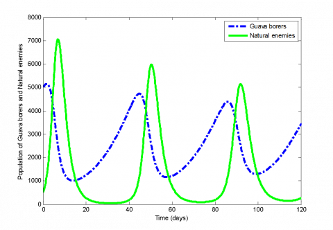
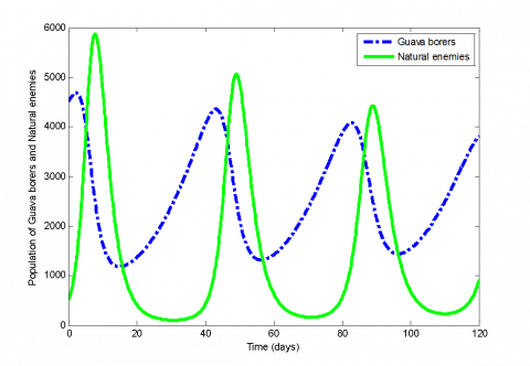
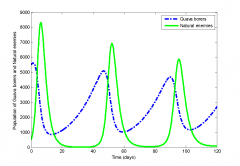
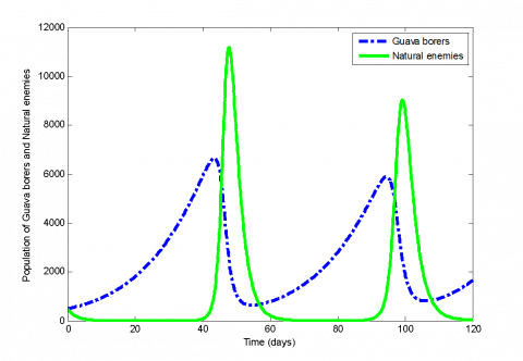
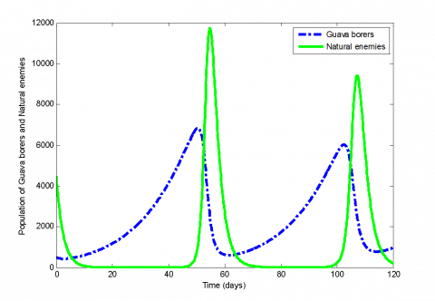
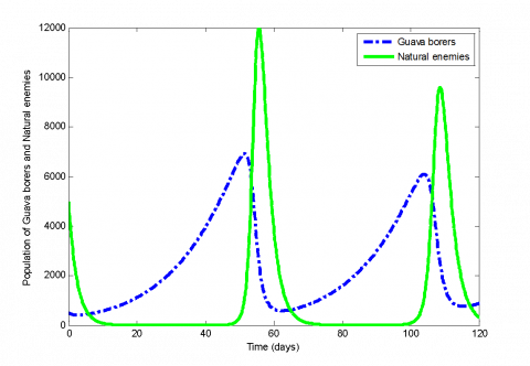
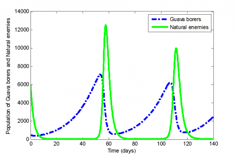
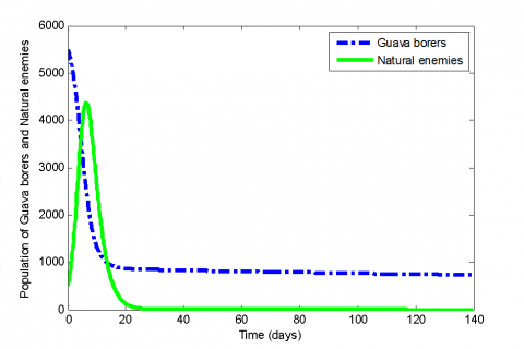
Figure 1. Population of Guava borers ( $x$ ) and natural enemies ( $y$ ) for initial values $x_{0}=5000$ and $y_{0}=500$ when $r=0.07$ , $a=0.0000020$ , $b=0.000046$ , $c=0.0002$ and $s=0.5$ . Here we have taken the time interval from 0 to 140
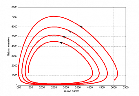
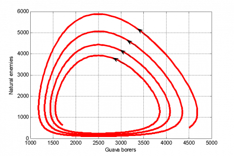
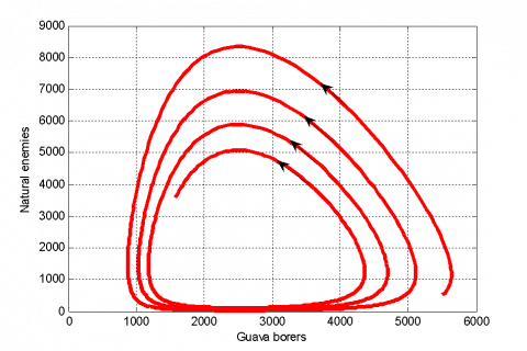
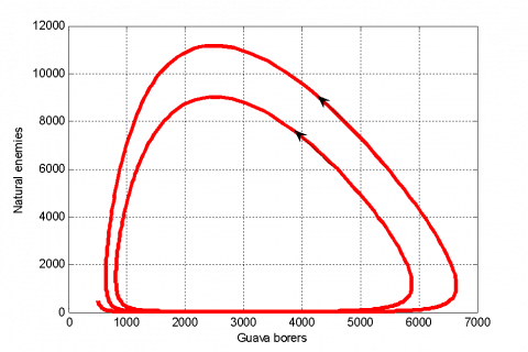
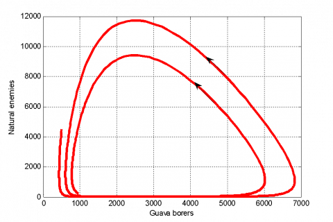
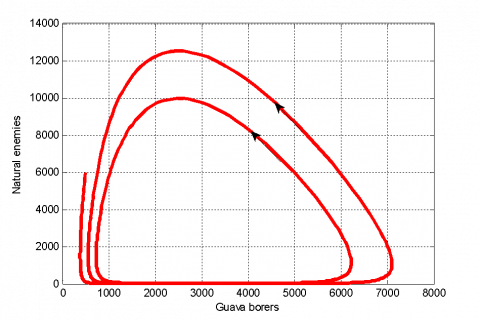
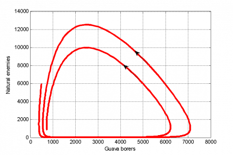
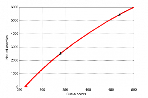
Figure 2. Phase portrait of population of Guava borers ( $x$ ) and natural enemies ( $y$ ) for initial values $x_{0}=5000$ and $y_{0}=500$ when the time interval from 0 to 140
In Figure 1, we consider the initial values of guava borers ( $x$ ) is 5000 and natural enemies ( $y$ ) is 500 where, $x$ denotes the number of guava borers and $y$ denotes the number of natural enemies. Here, we consider the time interval as days from 0 to 140. When $t=10$ , the figure shows the populations of borers are 1000 and population of natural enemies are 7000. That means the population of natural enemies increase and the population of guava borers decreases. Again at $t=40$ , the value of $x$ is 4500 and the value of $y$ is 100. That means, $y$ is decreasing as well as $x$ is increasing. It is observed that, at $t=0$ , the guava borers ( $x$ ) are 5000 and at $t=40$ , the guava borers ( $x$ ) are 4500. So, we can say that, the number of borer is gradually decreasing. But at terminal point when $t=140$ , borers population is 1.42×10³ and natural enemy’s population is 1.25×10³ . Finally, it is seen that, the number of borers are greater than the number natural enemies.
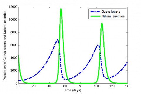
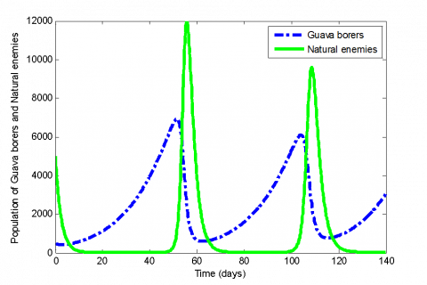
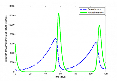
Here we see that, Figure 3 is similar to Figure 1 in 120 days. In the above figure (Figure 3) we take the time interval from 0 to 120. When, $t=120$ the borer’s population is $x$ = 3.43×10³ and the population of natural enemies are $y$ = 268.3166 .
Figure 3. Population of Guava borers ( $x$ ) and natural enemies ( $y$ ) for initial values $x_{0}=5000$ and $y_{0}=500$ when $r=0.07$ , $a=0.0000020$ , $b=0.000046$ , $c=0.0002$ and $s=0.5$ . Here we have taken the time interval from 0 to 120
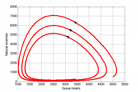
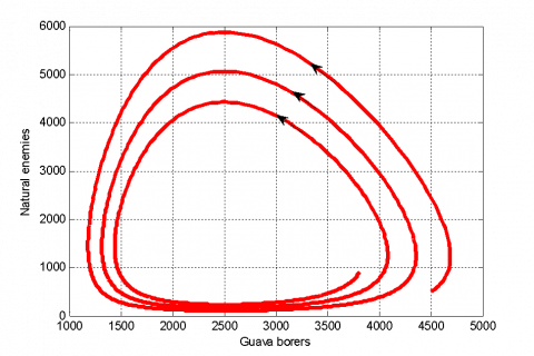
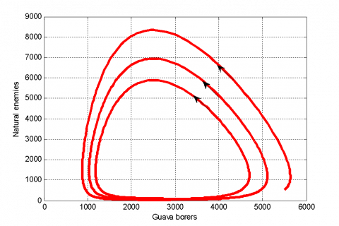
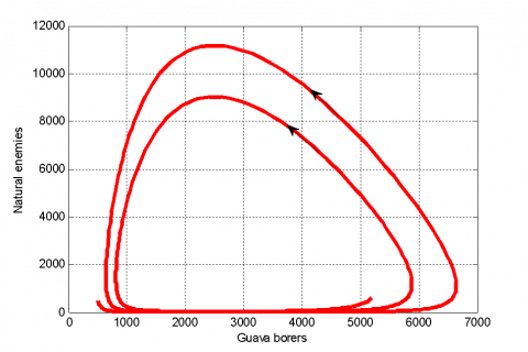
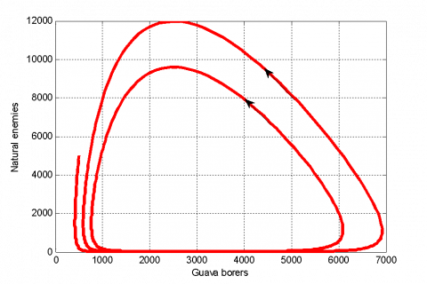
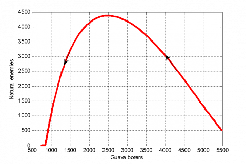
Figure 4. Phase portrait of population of Guava borers ( $x$ ) and natural enemies ( $y$ ) for initial values $x_{0}=5000$ and $y_{0}=500$ when the time interval from 0 to 120
If we compare the figures 1 and 3, we see that at 120th day (Figure 3) the borers population ( $x$ ) is much larger than the natural enemy’s population ( $y$ ). At 140th day (Figure 1) the value of $x$ and $y$ are closer than the value of $x$ and $y$ in Figure 3. That means it is more beneficial for the farmers to pluck the fruit at 140th day. Because at 140th day (Figure 1), the number of guava borers are less than the number of guava borers at 120th day (Figure 3).
Figure 2 and 4 is the phase portrait of the model for 140 and 120 days respectively. The behavior of all parameter values is oscillatory. We observe that the solutions are periodic and the periodic solutions are orbitally stable. The periodic time in Figure 2 is less than the periodic time in Figure 4. So the growth rate of guava is better for 0 to 120 days than the interval 0 to140 days. But without natural treatment, the more stable situation for the interval 0 to 140 days. The guava borers gradually decrease and increase with respect to natural enemies. The area in the middle of the figure shows the asymptotically stable region.
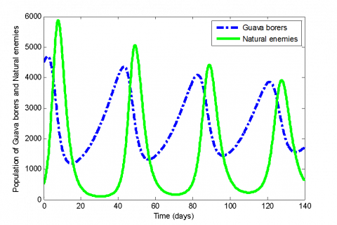
Figure 5. Population of Guava borers ( $x$ ) and natural enemies ( $y$ ) for initial values $x_{0}=4500$ and $y_{0}=500$ when $r=0.07$ , $a=0.0000020$ , $b=0.000046 a$ , $c=0.0002$ and $S=0.5$ . Here we have taken the time interval from 0 to 140
Figure 6. Phase portrait of population of Guava borers ( $x$ ) and natural enemies ( $y$ ) for initial values $x_{0}=4500$ and $y_{0}=500$ when the time interval from 0 to 140
Figure 5 is started with the values $x_{0}=4500$ and $y_{0}=500$ . At 10th day, we get $x=3000$ and $y=6000$ which shows that natural enemy’s population increases rapidly and guava borer’s population rapidly decreases. But, at 20th day, the value of $x$ is 1300 and $y$ is 500. This means in lack of guava borers the natural enemies decrease. When the natural enemies decrease the borer’s populations again increase. So the figure shows the competition between pest and natural enemies. At 140th day, $x$ = 1.71 × 10³ and $y$ = 617.9337 Finally, the populations of guava borers are larger than the populations of natural enemies.
Figure 7 is similar to Figure 5 for the time interval 120 days. We have taken the time interval 0 to 120 in Figure 7. At $t=120$ , we get $x$ = 3.813 ×10³ and $y$ = 911.4765
Figure 7. Population of Guava borers ( $x$ ) and natural enemies ( $y$ ) for initial values $x_{0}=4500$ and $y_{0}=500$ when $r=0.07$ , $a=0.0000020$ , $b=0.000046$ , $c=0.0002$ and $s=0.5$ . Here we have taken the time interval from 0 to 120
Figure 8. Phase portrait of population of Guava borers ( $x$ ) and natural enemies ( $y$ ) for initial values $x_{0}=4500$ and $y_{0}=500$ when the time interval from 0 to 120
Comparing Figures 5 and 7, we get that Figure 7 shows the better positions of $x$ and $y$. At 140th day, $x$ = 1.71 × 10³ and $x$ = 3.813 × 10³ at $t=120$ . So we observe that if the farmers collect the fruits at 140th day, they will be benefitted.
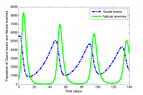
In Figure 9, at $t=40$ , we have got $x=5000$ and $y=10$ But at $t=50$ , we get $x=3000$ and $y=7000$ . That means when $x$ value increases, natural enemies also increase. At $t=90$ , we get $x=4800$ and $y=5500$ .That means, when natural enemies increase, borers decrease. Finally, at $t=140$ , the total number of guava borers are $x=1.57 \times 10^{3}$ and natural enemies are $y=3.57 \times 10^{3}$ So, the populations of natural enemies are larger than the population of guava borers. Figure 11 is similar to Figure 9 for 120 days. At $t=120$ , we get $x=2.73 \times 10^{3}$ and $y=106.8028$ . Comparing Figure 9 and Figure 11, we have got the best result for 140 days (Figure 9). If the farmers pick up the fruits at 140th day, they can receive the quality food than other days.
Figure 9. Population of Guava borers ( $x$ ) and natural enemies ( $y$ ) for initial values $x_{0}=5500$ and $y_{0}=500$ when $r=0.07$ , $a=0.0000020$ ,$b=0.000046$ , $c=0.0002$ and $s=0.5$ . Here we have taken the time interval from 0 to 140
Figure 10. Phase portrait of population of Guava borers ( $x$ ) and natural enemies ( $y$ ) for initial values $x_{0}=5500$ and $y_{0}=500$ when the time interval from 0 to 140
Figure 11. Population of Guava borers ( $x$ ) and natural enemies ( $y$ ) for initial values $x_{0}=5500$ and $y_{0}=500$ when $r=0.07$ , $a=0.0000020$ , $b=0.000046$ , $c=0.0002$ and $s=0.5$ . Here we have taken the time interval from 0 to 120
Figure 12. Phase portrait of population of Guava borers ( $x$ ) and natural enemies ( $y$ ) for initial values $x_{0}=5500$ and $y_{0}=500$ when the time interval from 0 to 140
Figure 13. Population of Guava borers ( $x$ ) and natural enemies ( $y$ ) for initial values $x_{0}=500$ and $y_{0}=500$ when $r=0.07$ , $a=0.0000020$ , $b=0.000046$ , $c=0.0002$ and $s=0.5$ . Here we have taken the time interval from 0 to 140
Figure 14. Phase portrait of population of Guava borers ( $x$ ) and natural enemies ( $y$ ) for initial values $x_{0}=500$ and $y_{0}=500$ when the time interval from 0 to 140
Figure 15. Population of Guava borers ( $x$ ) and natural enemies ( $y$ ) for initial values $x_{0}=500$ and $y_{0}=500$ when $r=0.07$ , $a=0.0000020$ , $b=0.000046$ , $c=0.0002$ and $s=0.5$ . Here we have taken the time interval from 0 to 120
Figure 16. Phase portrait of population of Guava borers ( $x$ ) and natural enemies ( $y$ ) for initial values $x_{0}=500$ and $y_{0}=500$ when the time interval from 0 to 120
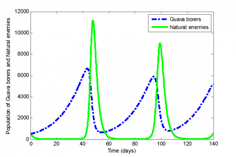
Figure 17. Population of Guava borers ( $x$ ) and natural enemies ( $y$ ) for initial values $x_{0}=500$ and $y_{0}=4500$ when $r=0.07$ , $a=0.0000020$ , $b=0.000046$ , $c=0.0002$ and $s=0.5$ . Here we have taken the time interval from 0 to 140
In Figure 13, at 50th day we get, $x=11500$ and $y=2000$ . At $t=100$ , we get $x=10000$ and $y=6000$ . Hence we see the interaction between guava borers and natural enemies. At time $t=120$ , $x$ value is 1.67 × 10³ and $y$ value is 32.5099 .
Figure 13 and 15 are similar to each other for 120 days. At $t=120$ , we get $x$ = 5.2022 × 10³ and $y$ = 587.5246 .In figure 13, at 50th day we get, $x$ = 11500 and $y$ = 2000 . At $t=100$ , we get $x$ = 10000 and $y$ = 6000 . Hence we see the interaction between guava borers and natural enemies. At time $t=120$ , $x$ value is 1.67× 10³ and $y$ value is 32.5099 .Comparing Figures 13 and 15, we get better result for 140 days (Figure 13).
In Figure 17, we see that initially borers population are increasing and natural enemies are decreasing. At $t=55$ , we get, $x$ = 1000 and $y$ = 11800. That means again $x$ is decreasing and $y$ is increasing. Finally, at $t=140$ , we get $x$ = 3.376 × 10³ and $y$ = 21.965.Figure 19 is similar to Figure 17 for 120 days. At $t=120$ , we get $x$ = 970.3620 and $y$ = 209.8794 Comparing the Figure 17 and 19, we get better result for 120 days (Figure 19).
Figure 18. Phase portrait of population of Guava borers ( $x$ ) and natural enemies ( $y$ ) for initial values $x_{0}=500$ and $y_{0}=4500$ when the time interval from 0 to 140
Figure 19. Population of Guava borers ( $x$ ) and natural enemies ( $y$ ) for initial values $x_{0}=500$ and $y_{0}=4500$ when $r=0.07$ , $a=0.0000020$ , $b=0.000046$ , $c=0.0002$ and $s=0.5$ . Here we have taken the time interval from 0 to 120
Figure 20. Phase portrait of population of Guava borers ( $x$ ) and natural enemies ( $y$) for initial values $x_{0}=500$ and $y_{0}=4500$ when the time interval from 0 to 140
Figure 21. Population of Guava borers ( $x$ ) and natural enemies ( $y$ ) for initial values $x_{0}=500$ and $y_{0}=5000$ when $r=0.07$ , $a=0.0000020$ , $b=0.000046$ , $c=0.0002$ and $s=0.5$ . Here we have taken the time interval from 0 to 140
In Figure 21, we see that initially guava borers population are increasing and natural enemy’s population are decreasing. At $t=55$ , we get, $x$ = 4000 and $y$ = 12000. That means, again $x$ is decreasing and $y$ is increasing. Finally, at $t=140$ , we get $x$ = 3.049 × 10³ and $y$ = 15.555.
Figure 22. Phase portrait of population of Guava borers ( $x$ ) and natural enemies ( $y$ ) for initial values $x_{0}=500$ and $y_{0}=5000$ when the time interval from 0 to 140
Figure 23. Population of Guava borers ( $x$ ) and natural enemies ( $y$ ) for initial values $x_{0}=500$ and $y_{0}=5000$ when $r=0.07$ , $a=0.0000020$ , $b=0.000046$ , $c=0.0002$ and $s=0.5$ . Here we have taken the time interval from 0 to 120
Figure 24. Phase portrait of population of Guava borers ( $x$ ) and natural enemies ( $y$ ) for initial values $x_{0}=500$ and $y_{0}=5000$ when the time interval from 0 to 140
Figure 23 is similar to Figure 21. At $t=120$, we get $x$ = 879.2025 and $y$ = 325.3513 .
Figure 25. Population of Guava borers ( $x$ ) and natural enemies ( $y$ ) for initial values $x_{0}=500$ and $y_{0}=6000$ when $r=0.07$ , $a=0.0000020$ , $b=0.000046$ , $c=0.0002$ and $s=0.5$ . Here we have taken the time interval from 0 to 140
Figure 26. Phase portrait of population of Guava borers ( $x$ ) and natural enemies ( $y$ ) for initial values $x_{0}=500$ and $y_{0}=6000$ when the time interval from 0 to 140
Figure 27. Population of Guava borers ( $x$ ) and natural enemies ( $y$ ) for initial values $x_{0}=500$ and $y_{0}=6000$ when $r=0.07$ , $a=0.0000020$ , $b=0.000046$ , $c=0.0002$ and $s=0.5$ . Here we have taken the time interval from 0 to 120
.
Figure 28. Phase portrait of population of Guava borers ( $x$ ) and natural enemies ( $y$ ) for initial values $x_{0}=500$ and $y_{0}=6000$ when the time interval from 0 to 120
Comparing the figures 21 and 23, we get better result for 120 days (Figure 23). In Figure 25, we see that initially guava borers population are increasing and natural enemy’s population are decreasing. At $t=57$ , we get, $x$ = 3500 and $y$ = 12500 . That means again $x$ is decreasing and $y$ is increasing. Finally, at $t=140$ , we get $x$ = 2.464 × 10³ and $y$ = 15.555. We show that, Figure 27 is similar to Figure 25 for 120 days. But we have taken the time interval 0 to120 in Figure 27. At $t=120$ we the values $x$ = 745.5455 and $y$ = 860.5480 . Comparing Figures 25 and 27, we can say that, if the farmers pick off the fruits at 120th day (Figure 27), they will be benefitted.
Figure 28 and 26 is the phase portrait of the model for 120 and 140 days. The behavior of all parameters values is oscillatory. We observe that the solutions are periodic and the periodic solutions are orbitally stable. The periodic time in Figure 28 is less than the periodic time in Figure 26. So, we get the better result for 120 days.
Here, we have analyzed the modified model to calculate the numerical results. we have taken the time interval from 0-120 days and 0-140 days as before. We use MATLAB (R2010a) to simulate the numerical results of this model by Runge-kutta method.
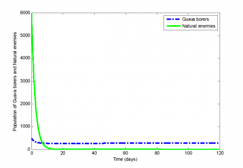
Figure 29. Population of Guava borers ( $x$ ) and natural enemies ( $y$ ) for initial values $x_{0}=5500$ and $y_{0}=500$ when $r=0.07$ , $a=0.0000020$ , $b=0.000046$ , $c=0.0002$ and $s=0.5$ . Here we have taken the time interval from 0 to 140
In Figure 29, we consider the initial values of guava borers are $x_{0}=5500$ and natural enemies are $y_{0}=500$ where, $x$ denotes the number of guava borers and $y$ denotes the number of natural enemies. Here, we consider the time interval as days from 0 to 140. When $t=10$ , the figure shows the population of borers ( $x$ ) are 4000 and population of natural enemies ( $y$ ) are 4500. That means the population of natural enemies increase and the population of guava borers decreases. Again, at $t=20$ , the value of $x=1000$ and the value of $y=50$ . That means $y$ is also decreasing as well as $x$ is decreasing. It is observed that, $t=0$ , the $x$ value is 5500 and at $t=20$ , the $x$ value is 4.4.1000. So, we can say that, the number of borer is gradually decreasing. But at terminal point when time is 140, borer’s population is 730.2053 and natural enemy’s population is 1.744 × 10⁻¹⁶ . Finally, in this figure the population of guava borers is controlled. The solutions of phrase portrait are not periodic and the solutions are gradually stable. The initial number of guava borers is 5500 and natural enemies are 500. When $x=4000$ , we get from figure the value of $y$ is 3000. That means using this natural treatment borers population is decreasing and natural enemy’s population is also decreasing. Finally, the number of guava borers is decreased.
Figure 30. Phase portrait of population of Guava borers ( $x$ ) and natural enemies ( $y$ ) for initial values $x_{0}=5500$ and $y_{0}=500$ when the time interval from 0 to 140
Comparing Figures 9 and 29, we observe that the borer’s population (Figure 9) is 1.57 × 10³ and the population of borers (Figure 29) is 730.2053. Clearly, it is seen that there is a massive reduction of guava borer’s population. So, we can say that, if the farmers use the natural treatment (spraying of neem leaves) on guava fruit they can be more benefitted.
Figure 31. Population of Guava borers ( $x$ ) and natural enemies ( $y$ ) for initial values $x_{0}=500$ and $y_{0}=6000$ when $r=0.07$ , $a=0.0000020$ , $b=0.000046$ , $c=0.0002$ and $s=0.5$ . Here we have taken the time interval from 0 to 120
In Figure 31, we consider the initial values of guava borers are $x_{0}=500$ and natural enemies are $y_{0}=6000$ Here, we consider the time interval as days from 0 to 120. When $t=10$ , the figure shows the population of borers ( $x$ ) are 300 and population of natural enemies ( $y$ ) are 50. That means the population of natural enemies decrease and the populations of guava borers also increase. It is observed that, $t=0$ , the $x$ value is 500 and at $t=10$ , the $x$ value is 300. So, we can say that, the number of borer is gradually decreasing. But at terminal point when $t=120$ , borers population is 3.334 × 10⁻²⁰ and natural enemy’s population is 268.7349. Finally, in this figure the population of guava borers is controlled. The solutions of phase portrait are not periodic and the solutions are gradually stable. The initial population of guava borer is 500 and natural enemies are 6000. When the number of guava borer is 400, the number of natural enemies is 400. And at the end, guava borers are decreased and controlled.
Comparing Figures 27 and 31, we get the value of $x$ in Figure 27 is 745.5454 and the value of $x$ in Figure 31 is 268.7349 . So, using natural treatment (spraying of neem leaves) is more profited for guava farmers.
Figure 32. Phase portrait of population of Guava borers ( $x$ ) and natural enemies ( $y$ ) for initial values $x_{0}=500$ and $y_{0}=6000$ when the time interval from 0 to 140
Natural treatment (spraying of neem leaves) on guava fruit save fruit from borer and human healh from side effect of chemical while minimizing the cost of treatment in the presence of natural enemies (parasitoids). We observe that it is a good harvesting time at 140 days for some initial values (when the number of initial values of guava borers are greater than the number of initial values of natural enemies) and we also get a good harvesting time at 120 days for some another initial values (when the number of initial values of natural enemy are greater than the number of initial values of guava borer) in our actual model. But if we compare between the actual model and the modified model, we see that, our modified model that means natural treatment on guava is more preferable than the actual model. Because at 120-140 days, the modified model shows the better results for any initial values of guava borer and natural enemy than our actual model. This modified model is not harmful for animals or nature. We believe that the results of the modified model can help the farmer to save the guava borer and it is also health benefitted for human.
We thanks the officers of agriculture and some farmers for their useful suggestions which have improved the quality of this paper.
[1] Anisiu MC. (2014). Lotka, volterra and their model. Didactica Mathematica 32: 9-17.
[2] BBS. (2017). Yearbook of Agricultural statistics (2016). Bangladesh Bureau of statistics (BBS), Ministry of Planning, Government of the People’s Republic of Bangladesh, Dhaka.
[3] Dym CL. (2004). Principles of mathematical modeling. 2th edition, Elsevier Academic Press, Burlington, USA.
[4] Kar TK. (2005). Stability analysis of a Prey- Predator model incorporating a prey refuge. Communications in Nonlinear Science and Numerical Simulations 10: 681-691. http://dx.doi.org/10.1016/j.cnsns.2003.08.006
[5] Lotka AI. (1927). Fluctuation in the abundance of the species considered mathematically (with comment by Voltra, V). Nature 119: 12-13. http://dx.doi.org/10.1038/119012a0
[6] Mallick UK, Biswas MHA. (2017). Optimal control strategies applied to reduce the unemployed population. In: Proceeding of 5th IEEE R10-HTC, BUET, Dhaka, 21-23 December, 408-411
[7] Murray JD. (2002). Mathematical biology, 3th edition, Springer, New York.
[8] NIPHM (2014). Aisa based IPM package. Department of agriculture and Cooperation, Ministry of Agriculture, Government of India.
[9] Obabiyi OS, Olaniyi S. (2013). Mathematical model for malaria transmission dynamics in human and mosquito populations with nonlinear force of infection. International Journal of Pure and Applied Mathematics 88: 22-32.
[10] Pantha G. (2015). A mathematical model for unemployment with effect of self-employment. IOSR Journal of Mathematics 11: 37-43. http://dx.doi.org/10.9790/5728-11613743
[11] Perko L. (2001). Differential equations and dynamical systems. 3th edition, Springer-Verlag, Inc., New York.
[12] Rafikov M. (2009). Optimization of biological pest control of sugarcane borer. 18th IEEE International Conference on Control Applications, Part of 2009 IEEE Multi-conference on Systems and Control, IEEE, Saint Petersburg, Russia, July 8-10. http://dx.doi.org/10.1109/CCA.2009.5280989
[13] Rafikov M, Balthazar JM, Bremen HFV. (2007). Mathematical modeling and control of population systems: Application in biological pest control. Applied Mathematics and Computation 200: 557-573. http://dx.doi.org/10.1016/j.amc.2007.11.036
[14] Rafikov M, Balthazar JM. (2005), Optimal pest control problem in population dynamics. Computational and Applied Mathematics 24(1): 65-81. http://dx.doi.org/10.1590/S0101-82052005000100004
[15] Sharma A, Diwevidi VD, Singh S. (2013). Biological pest control and its importance in agriculture. International Journal of Biotechnology and Bioengineering Research 4(3): 175-180.
[16] Singh AK, Misra AK. (2010). A mathematical model for unemployment. Nonlinear Analysis: Real World Applications 12(1): 128-136.
[17] Shen J, Tang S, Xu C. (2017). Analysis and research on home-based care for the aged based on insurance policy under government leading. AMSE Journals-AMSE IIETA-Series: Advances A 54(1): 106-126.
[18] Thomas MB, Willis AJ. (1998). Biocontrol- risky but Necessary. Trends in Ecology and Evolution 13: 325-329.
http://dx.doi.org/10.1016/S0169-5347(98)01417-7
[19] Vasishtha AR. (2004). Numerical analysis. 4th edition, Kedar Nath Ram Nath, Mecut College, Meerut.
[20] Qu W, Xie Y, Shen Y, Han J, You M, Zhu T. (2017). Simulation on the effects of various factors on the motion of ultrasonic cavitation bubble. Mathematical Modelling of Enineering Problems 4(4): 173-178. https://doi.org/10.18280/mmep.040406