Hai Gu | Jie Gao | Yuwei Yang | Xiuwei Fu*
© 2023 IIETA. This article is published by IIETA and is licensed under the CC BY 4.0 license (http://creativecommons.org/licenses/by/4.0/).
OPEN ACCESS
While designing the inverter, the total harmonic distortion (THD) in the output is a major concern to decide its performance. In order to calculate the total harmonic distortion (THD) of a symmetric modular multilevel inverter (MMI) with switched capacitors, a Harris hawk optimization (HHO) was used in this study. Utilizing symmetric and identical DC sources, the suggested modular multilevel inverter is designed. The suggested topology may be expanded up to many levels and utilizes fewer switches to provide 9 levels of output than conventi1al cascaded H-bridge multilevel inverters. Using a low-frequency switching control approach known as selective harmonic elimination pulse width modulation, the switches are less stressed and the inverter output's THD profile is improved. Additionally, the switching angles of the MMI have been optimized by solving the non-linear equations of the SHEPWM using the Harris Hawk Optimizer. Ant colony optimization (ACO) and particle swarm optimization (PSO), two alternative optimizers, were compared in terms of the THD of the output. This comparison shows that the HHO delivers a lower THD than other optimization techniques approximately near to 5%, as per the IEEE-519 standard, and is thus more highly advised. Finally, a hardware configuration for the suggested inverter is implemented to confirm the simulation findings.
single chamber two-population microbial fuel cell, additive manufacturing, nonlinear model, fault detection, observer, LMI, uncertainty, adaptive approach.
Energy is the most important factor of development and one of the main factors of production that has a direct impact on the quality of life of people and the development of communities. With the aim of providing adequate and satisfactory energy, various studies in the field of energy systems are underway [1-3]. Due to environmental benefits, improved energy security, diversity in energy production methods, flexibility in energy exchanges and many other capabilities, the share of renewable energy in the overall energy portfolio is increasing. At the same time, increasing the efficiency of energy received from renewable sources has doubled their popularity. Despite the high cost of these systems, because of the straight impact on human health and with the purpose of sustainable development, investment and development of these systems have been quite reasonable. Therefore, optimal management and planning of these sustainable energy sources is one of the main approaches in various studies [6-8].
Fuel cell is extremely important among renewable energy sources due to its energy production, effective performance in the field of wastewater treatment, pollution reduction and multifunctional potential, and plays an important role in both energy and the environment [9]. One of the most common and well-known technologies related to fuel cells for power generation and wastewater treatment is microbial fuel cell (MFC) [10-12]. This type of fuel cell is a subset of biomass that generates electrical energy by trapping electrons metabolized by specific microorganisms in wastewater, and reduces carbon dioxide in the atmosphere by treating wastewater. Notably, various researches are being conducted on it from different perspectives. Most of the investigations have been done on improving the physical modules of MFC, MFC planning, linking MFC with other technologies and obviously optimal control of MFC. Additive manufacturing (AM) techniques are a new and attractive technology for producing materials with complex structures. Additive manufacturing is a useful technology for manufacturing energy converters and a promising aspect for fuel cells for clean energy conversion with low-cost geometric structures for assembling fuel cell components. AM techniques being also suitable for generating microstructures and flexible electrochemical active regions of fuel cells with high precision and resolution that provide the following opportunities: (1) minimizing fabrication time, (2) reducing material waste, (3) complex structure engineering, (4) cost-effectiveness, and environmentally friendly processing. However, very restricted exploration has been done on fault study in MFCs [13-15]. In general, fault analysis in various systems is extremely important, because it can greatly increase the reliability and safety of technical processes and avoid the instability of the closed-loop system. Early detection of faults can also prevent abnormal process progress, decrease productivity and production losses, and empower the planning and execution of smart measures to avoid system catastrophic failures [16]. Therefore, fault identification and analysis are essential for the effective and safe operation of the MFC.
As a consequence of the presence of microorganisms, complex configuration and tough coupling properties in MFC [17-18], the incidence of fault is high, even though its diagnosis is very difficult. Various types of faults can be observed in MFC, including low substrate utilization, low microbial activity, lack of oxygen, decreased substrate concentration, and sensor defects. Thus, to achieve stable and reliable performance as well as to prevent possible damages, this study was conducted with the aim of rapid fault identification in MFC.
Deep learning and wavelet packet techniques are the most important procedures for detecting faults in microbial fuel cells, but each has its own drawbacks. The former offers effective performance in data classification, but suffers from the complexity of the mechanism, as well as the high volume of calculations and the very high volume of data [19]. The latter is not able to detect types of faults online despite being able to detect different types of faults [20]. The practical implementation of the Q-tree fault detection technique evaluated in reference [21] has not yet been possible. The inclusion of issues related to the consideration of parameter uncertainty and nonlinear model in the MFC fault detection technique has remained barren so far. Parameter uncertainty, which is often present in the modeling of physical systems, and is also true of MFCs [22-23], has not been considered in any of the MFC faults studies to date. Linear models, linearization or elimination of nonlinear terms in MFC fault detection also have their own shortcomings in modeling and defect identification.
So, the most important innovation of this paper is to present a robust fault detection scheme considering the inconveniences of nonlinear MFC system and parametric uncertainty. First, a two-population nonlinear MFC model is planned to accurately describe the system dynamics and achieve effective and precise information about the MFC system, and then parametric uncertainty is included in the model. By designing a hybrid technique based on linear matrix inequality (LMI) and adaptive approaches, a novel robust observer is introduced for fault detection in the MFC system, in which the upper bound of uncertainty is considered unknown. By solving the linear matrix inequality and by means of the adaptive technique, the physical solution to the problem of fault detection is obtained in a nonlinear MFC system with two populations at any time and it can be used for additional processing.
This article is as follows; In the second part, the MFC builtup methods based on additive manufacturing are described firt, and then the nonlinear model of the MFC system is offered. In this section, uncertainties in the model along with various parameters of MFC are described. The third section describes the diagnostic scheme. This technique is fully explained by considering the working class that takes in the MFC model. The fourth section gives the simulation results and the fifth section presents the conclusions.
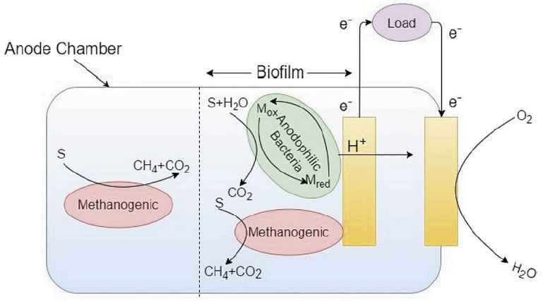
AM technologies are included in the following groups: 1- binder jetting; 2- vat polymerization; 3- material extrusion; 4- powder bed fusion (PFB); 5- material jetting; 6- sheet lamination; and 7- directed energy deposition. The first four methods of AM technologies are used in fuel cell manufacturing and the rest of them, despite having a high potential, are still under research and development. In MFC, the anode plays an important role and acts both as a conductor and as a carrier of bacteria. The selective laser melting-based AM method has been used to fabricate the aluminum alloy anode with higher power [24] and the selective laser sintering method has been used to fabricate the anode with low density, high surface area, and ideal surface roughness. In MFC, the proton exchange membrane is another main component, and Polyjet 3D printing technology which belongs to the material extrusion category, has been used to make the Tangoplus polymer ion exchange membrane [25] which has a large surface area and is less prone to biodegradation and biofouling, providing longer lifetime and higher power output for operation. A high-performance membrane of Gel-Lay and large anode surface has also been fabricated using fused deposition modeling (FDM) [26] and it has been proven that AM is able to fabricate more than one functional component in a microbial fuel cell. In [27], FDM was used to fabricate a single-chamber air-cathode microbial fuel cell without supporting fixtures, fittings, and gaskets. Simplifying the manufacturing process, reducing the size and thus increasing the surface area, increasing the power density, longer lifetime for operation, lower biodegradation and biofouling and processing of inexpensive materials such as thermoplastics are among the advantages of using additive manufacturing technology for the MFC system. Figure 1 shows the structure of a microbial fuel cell. The anode, cathode, membrane, substrate and bacterial species are the main components of the MFC system. First, the electrons produced by the microorganisms are transferred directly or through an external medium to the MFC anode electrode. They are then transferred to the MFC cathode via an external circuit, where they combine with receptor electrons such as oxygen or ferricyanide. During this process, in addition to extracting electrical power, wastewater is also treated. The overall performance of MFCs and microbial systems depends on many components. A nonlinear model describing the dynamics of the MFC system is now presented, and this model is used to design an unknown input observer. For a singlechamber two populations MFC, a model with parameterized uncertainty is as follows:
$\dot{x}_1=\theta_1 \frac{x_3}{k_a+x_3} x_1-k_a x_1-a_a d x_1$ (1)
$\dot{x}_2=\theta_2 \frac{x_3}{k_\beta+x_3} x_2-k_d x_2-a_m d x_2$ (2)
$\dot{x}_3=-k_1 \theta_1 \frac{x_3}{k_a+x_3} x_1-k_2 \theta_2 \frac{x_3}{k_\beta+x_3} x_2 +d\left[u(t)-x_3\right]$ (3)
Figure 1. Single Chamber two-population MFC
where, x1, x2 and x3 are the anodophilic, methanogenic microorganisms acetate (substrate) concentration, in that order. Input u is the influent substrate concentration (So), and the dilution rate d specifies the ratio of the input flow rate of substrate to the volume of the chamber. This parameter is an important feature to adjust the growth rate of microorganisms [28]. On the other hand, to avoid the necessity for big control action, influent concentration (So) is considered as an input for satisfying the control objective. The parameters of k1 and k2 are the reciprocals of anodophilic and methanogenic bacterial, in that order. The $\left(\boldsymbol{k}_{\boldsymbol{a}}\right)$ and $\left(\boldsymbol{k}_{\boldsymbol{\beta}}\right)$ are decay rates of anodophilic and methanogenic microorganisms, respectively. Also, $a_a$ and $a_m$ are bio-film retention constants. Parameters $\boldsymbol{\theta}_1$ and $\boldsymbol{\theta}_2$ are $\boldsymbol{\mu}_{\boldsymbol{m a x}, \boldsymbol{a}}, \,\,\boldsymbol{r}\left(\boldsymbol{M}_{\boldsymbol{o}}\right)$ and $\boldsymbol{\mu}_{\boldsymbol{m a x}, \boldsymbol{m}}$ in that order, which in company with other parameters are fully explained in [22].
This part provides the organization of the fault detection technique for the nonlinear model of MFC. The MFC model is involved in the subsequent continuous nonlinear system class
$\begin{gathered}\dot{x}(t)=A x(t)+B u(t)+g(x)+f(t) \\ y(t)=C x(t)\end{gathered}$ (4)
As stated by the MFC model, x(t) signifies the states of system and A and B indicate the matrixes of linear coefficients in Equation (4) and g(t) takes in the uncertainty of the model in addition to the nonlinear terms present in the system model.
$A=\left[\begin{array}{ccc}-k_a-a_a d & 0 & 0 \\ 0 & -k_d-a_m d & 0 \\ 0 & 0 & -d\end{array}\right]$
$B=\left[\begin{array}{l}0 \\ 0 \\ d\end{array}\right]$
$g(x)=\left[\begin{array}{c}\theta_1 \frac{x_3}{k_a+x_3} x_1 \\ \theta_2 \frac{x_3}{k_\beta+x_3} x_2 \\ -k_1 \theta_1 \frac{x_3}{k_a+x_3} x_1-k_2 \theta_2 \frac{x_3}{k_\beta+x_3} x_2\end{array}\right]$
y is the output of the system and ${f}(t)$ is the input fault to the system which follows the subsequent equation $f(t) \in R^{n_u}$ is fault in the system and ${f}(t)$ belong to
$F=\left\{f(t) \in R^{n_u} \mid\|f\| \leq f_{\max }\right\}$ (5)
where ${f}(t)$ is bounded and it is supposed that there is no information about its upper boundary $(f_{max})$. In other words, by designing of an unknown input observer to distinguish fault without knowledge from its upper bound, we are capable to recognize and detect any of MFC system faults with any amplitude.
The dynamics of the observer is now defined as follows:
$\dot{\hat{x}}(t)=A \hat{x}(t)+ B u(t)+g(\hat{x})+\hat{f}(t) +L(y(t)-\hat{y}(t))$
$\hat{y}(t) =C \hat{x}(t)$ (6)
where, $\hat{x}(t)$ specifies the observer states, $\hat{y}(t)$ indicates the observer output vector and $\hat{f}(t)$ also signifies the fault estimate.
By describing the error between the actual system and observer states as Equation (7), it is obtained
$e(t)=x(t)-\hat{x}(t)$ (7)
As well as defining the error between the actual value of the fault and its estimatin as follows
$\tilde{f}(t)=f(t)-\hat{f}(t)$ (8)
The error dynamics becomes as follows
$\dot{e}(t)=(A-L C) e(t)+g(x(t))-g(\widehat{x}(t))+\tilde{f}(t)$ (9)
Given that the Lipshitz condition is set to $g(x(t))$, the following relation can be written for it
$g(x(t))-g(\widehat{x}(t)) \leq \gamma|x(t)-\widehat{x}(t)|=\gamma e(t)$ (10)
Now, by placing the Lipshitz condition in Equation (10) in the system error equations (9), it is obtained:
$\dot{e}(t)=(A-L C+\gamma I) e(t)+\tilde{f}(t)$ (11)
Which I represents the unit matrix in the dimensions of the system states. Now to design the observer and also to ensure the stability of the system, Lyapunov function is scheduled in the following form:
$V(t)=e^T(t) P e(t)+\frac{1}{\eta} \tilde{f}^T \tilde{f}$ (12)
where, P is a positive symmetric matrix that is ultimately obtained by the LMI method and $\eta$ is also a positive parameter for regulating adaptive law. From Equation (12), we derive the first order to prove the stability of the observer.
${r}\dot{V}(t)=\dot{e}^T(t) P e(t)+e^T(t) P \dot{e}(t)-\frac{1}{\eta}\left(\dot{\hat{f}}^T \tilde{f}+\tilde{f}^T \dot{\hat{f}}\right)$ (13)
As we know, in order to guarantee stability, in addition to the Lyapunov function must be positive-definite, and this can be seen in Equation (12), the derivative of Lyapunov function must also be negative semi-definite, i.e.
$\dot{V}(\boldsymbol{t}) \leq \mathbf{0}$ (14)
To establish relation (14), it is necessary that
$\dot{e}^T(t) P e(t)+e^T(t) P \dot{e}(t)-\frac{1}{\eta}\left(\dot{\hat{f}}^T \tilde{f}+\tilde{f}^T \dot{\hat{f}}\right) \leq 0$ (15)
It is now obtained by placing Equation (11) in relation (15)
$((A-L C+\gamma I) e(t)+\tilde{f}(t))^T P e(t)+e^T(t) P((A-L C+\gamma I) e(t)+\tilde{f}(t))-\frac{1}{\eta}\left(\hat{\hat{f}}^T \tilde{f}+\tilde{f}^T \dot{\hat{f}}\right) \leq 0$ (16)
With a little mathematical simplification, Equation (16) is rewritten as follows:
$e^T(t)((A-L C+\gamma I)^T P+P(A-L C+\gamma I)) e(t)+e^T(t) P \tilde{f}+\tilde{f}^T P e(t)-\frac{1}{\eta}\left(\dot{\hat{f}}^T \tilde{f}+\tilde{f}^T \dot{\hat{f}}\right) \leq 0$ (17)
It is now obtained by factoring from $\tilde{f}$ and $\tilde{f}^T$ in Equation (17)
$e^T(t)((A-L C+\gamma \boldsymbol{I})^T P+P(A-L C+\gamma I)) \boldsymbol{e}(\boldsymbol{t})+\left(e^T(t) P-\frac{1}{\eta} \dot{\hat{f}}^T\right) \tilde{f}+\tilde{f}^T\left(P e(t)-\frac{1}{\eta} \dot{\hat{f}}\right) \leq \mathbf{0}$ (18)
It is clear that in order to eliminate the effects of the estimation error $\tilde{f}$ and $\tilde{f}^T$, the coefficients of these factors must be equal to zero in relation (18), and paying attention to this point gives the necessary settings as follows:
$e^T(t) P-\frac{1}{\eta} \dot{\hat{f}}^T=0$ (19)
$P e(t)-\frac{1}{\eta}\dot{\hat{f}}=0$ (20)
Solving each of Equation (19) or (20) gives:
$\dot{\hat{f}}=\eta P e(t)$ (21)
Equation (21) is in fact the adaptive law for estimating the fault entered into the system. It is obtained by placing Equation (21) in Equation (18)
$e^T(t)\left((A-L C+\gamma I)^T P\right.+P(A-L C+\gamma I)) e^T(t) \leq 0$ (22)
By means of multiplying $e^T(t)$ from the left and $e(t)$ from the right and substituting $P=X^{-1}, X>0$ and $L=Y X^{-1}$
$((A+\gamma I) X-Y C)^T+(A+\gamma I) X+Y C \leq 0$ (23)
$X>0$ (24)
Solving LMI (23) and (24) ensures the stability of the observer system. Therefore, the stability of fault observer is guaranteed and in the next part, we will evaluate its efficiency by performing simulations.
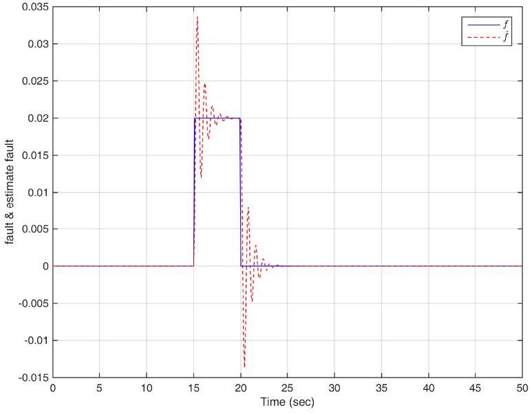
In this section, numerical simulation using MATLAB software is used to show the ability of the planned technique to precisely and rapidly detect the fault. It is assumed that an unknown input fault signal in the formula of (25) enters the MFC system.
$f(t)=\left\{\begin{array}{cc}0.02 & \text { if } t \geq 15 \text { and } t \leq 20 \\ 0 & \text { otherwise }\end{array}\right.$ (25)
By trial and error, the parameters related to the diagnostic technique are designated as follows:
$\gamma=10, \eta=10$ (26)
By substituting the parameters and solving the LMI in Equations (23) and (24), the P and L matrices are achieved as follows:
$L=\left[\begin{array}{lll}2.24 & 3.08 & 4.53\end{array}\right]^T$ (27)
$P=\left[\begin{array}{ccc}-15.56 & 8.18 & 8.09 \\ 8.18 & -15.09 & 7.95 \\ 8.09 & 7.95 & -14.35\end{array}\right]$ (28)
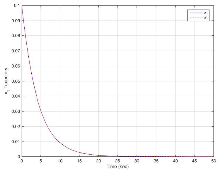
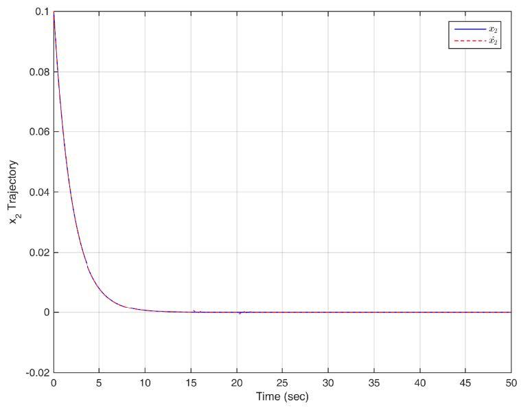
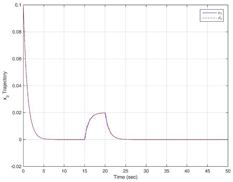
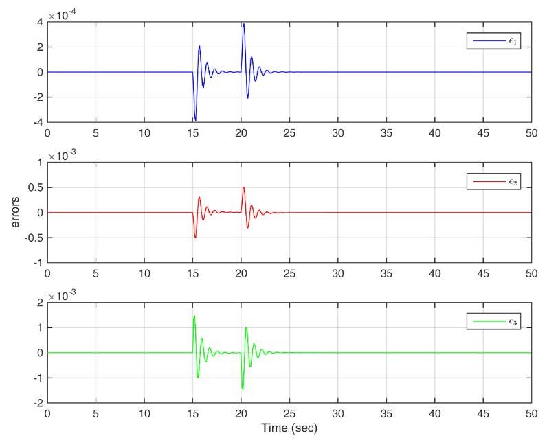
After applying the mentioned values to the observer and the error dynamics in Equations (21) and (11), the estimates of the states $x_1(t), x_2(t)$ and $x_3(t)$ of the microbial fuel cell system are obtained, as displayed in Figures 2 to 4. Figure 2 displays the trajectory of $x_1(t)$ and its estimation, whereas Figures 3 and 4 display the trajectories of $x_2(t)$ and $x_3(t)$ and their estimations, respectively. Figure 5 displays the quantity of error among the states and their estimations. It is obvious from the simulation results that in faultless periods, the planned observer is capable to precisely follow the fuel cell system states and the estimation error level is nearly zero. But after the error occurs, the estimation error increases which is obvious in Figure 5. As shown in Figure 6, the high speed of fault detection is another desirable feature for the planned unknown input observer.
Figure 2. Trajectory of $x_1(t)$
Figure 3. Trajectory of $x_2(t)$
Figure 4. Trajectory of $x_3(t)$
Figure 5. Observer error $e_1(t), e_2(t), e_3(t)$
Figure 6. Fault signal and its estimation
In this paper, a new scheme presented for fault diagnosis in a microbial fuel cell system. First, a nonlinear model of a fuel cell system was considered with first-order differential equations, in which both parametric uncertainties and nonlinear dynamics were embedded, and then a novel robust technique was designed for fault detection based on an unknown input observer. In the planned hybrid scheme, the adaptive technique and the linear matrix inequality approach were used simultaneously to ensure the stability of the observer error dynamics. By establishing Lipshitz conditions on the nonlinear dynamics of the microbial fuel cell system, even without knowing the uncertainty upper limit, the designed observer was able to quickly and accurately detect a fault in the system. The results of the numerical simulation in MATLAB software also established the the ability of the planned fault detection scheme. Fault detection in the presence of disturbances along with controlling its effects can be a good way for future studies in the field of microbial fuel cell system defects.
This work was financially supported by the funding for key research and cultivation projects of Nantong Institute of Technology (XKYPY202309, XKYPY202312), the Top Talent Project of Nantong Institute of Technology (XBJRC2021003), Key disciplines of the 14th five year plan in Jiangsu Province: Mechanical Engineering (2022-2), First-class specialty and industry education integration brand specialty in Jiangsu Province: Mechanical Design, Manufacturing and Automation (2020-9,2022-7), Science and technology project of Nantong (JC2020155).
|
THD |
Total Harmonic Distortion |
|
MMI |
Modular Multilevel Inverter |
|
PSO |
Particle swarm optimization |
|
ACO |
Ant Colony Optimization |
|
HHO |
Harris Hawk Optimization |
|
PWM |
Pulse Width Modulation |
|
SHEPWM |
Selective Harmonic Elimination PWM |
|
SVPWM |
Space Vector Pulse Width Modulation |
|
MLI |
Multilevel Inverter |
|
NPC |
Neutral Point Clamping |
|
FC |
Flying Capacitor |
|
CHB |
Cascaded H-Bridge |
|
NSwitch |
Number of Switches |
|
NGate |
Number of Gate Drivers |
|
NSource |
Number of DC Sources |
|
NDiode |
Number of Switched Diodes |
|
NDClink |
Number of DC link Capacitors |
|
TBlock |
Total Blocking Voltage |
[1] Perera, A. T. D., Javanroodi, K., & Nik, V. M. (2021). Climate resilient interconnected infrastructure: Cooptimization of energy systems and urban morphology. Applied Energy, 285, 116430.
[2] Härtel, P., & Korpås, M. (2021). Demystifying market clearing and price setting effects in low-carbon energy systems. Energy Economics, 93, 105051.
[3] Schweiger, G., Heimrath, R., Falay, B., O'Donovan, K., Nageler, P., Pertschy, R., ... & Leusbrock, I. (2018). District energy systems: Modelling paradigms and generalpurpose tools. Energy, 164, 1326-1340.
[4] Schmidt, J., Gruber, K., Klingler, M., Klöckl, C., Camargo, L. R., Regner, P., ... & Wetterlund, E. (2019). A new perspective on global renewable energy systems: why trade in energy carriers matters. Energy & Environmental Science, 12(7), 2022-2029.
[5] Østergaard, P. A., Johannsen, R. M., & Duic, N. (2020). Sustainable development using renewable energy systems. International Journal of Sustainable Energy Planning and Management, 29, 1-6.
[6] Eriksson, E. L. V., & Gray, E. M. (2019). Optimization of renewable hybrid energy systems–A multi-objective approach. Renewable energy, 133, 971-999.
[7] Zakaria, A., Ismail, F. B., Lipu, M. H., & Hannan, M. A. (2020). Uncertainty models for stochastic optimization in renewable energy applications. Renewable Energy, 145, 1543-1571.
[8] Elsheikh, A. H., & Abd Elaziz, M. (2019). Review on applications of particle swarm optimization in solar energy systems. International journal of environmental science and technology, 16(2), 1159-1170.
[9] Sharaf, O. Z., & Orhan, M. F. (2014). An overview of fuel cell technology: Fundamentals and applications. Renewable and sustainable energy reviews, 32, 810-853.
[10] Das, D. (2018). Microbial Fuel Cell (pp. 21-41). New Delhi, India: Springer.
[11] Rahimnejad, M., Adhami, A., Darvari, S., Zirepour, A., & Oh, S. E. (2015). Microbial fuel cell as new technology for bioelectricity generation: A review. Alexandria Engineering Journal, 54(3), 745-756.
[12] Gul, H., Raza, W., Lee, J., Azam, M., Ashraf, M., & Kim, K. H. (2021). Progress in microbial fuel cell technology for wastewater treatment and energy harvesting. Chemosphere, 130828.
[13] Mathuriya, A. S., Jadhav, D. A., & Ghangrekar, M. M. (2018). Architectural adaptations of microbial fuel cells. Applied microbiology and biotechnology, 102(22), 9419-9432.
[14] Sonawane, J. M., Gupta, A., & Ghosh, P. C. (2013). Multielectrode microbial fuel cell (MEMFC): a close analysis towards large scale system architecture. International journal of hydrogen energy, 38(12), 5106-5114.
[15] Fu, L., Fu, X., & Imani Marrani, H. (2022). Finite Time Robust Controller Design for Microbial Fuel Cell in the Presence of Parametric Uncertainty. Journal of Electrical Engineering & Technology, 17(1), 685-695.
[16] Ma, F., Lian, L., Ji, P., Yin, Y., & Chen, W. (2020). Fault Diagnosis Scheme Based on Microbial Fuel Cell Model. IEEE Access, 8, 224306-224317.
[17] Logan, B. E. (2008). Microbial fuel cells. John Wiley & Sons.
[18] Vinayak, V., Khan, M. J., Varjani, S., Saratale, G. D., Saratale, R. G., & Bhatia, S. K. (2021). Microbial fuel cells for remediation of environmental pollutants and value addition: special focus on coupling diatom microbial fuel cells with photocatalytic and photoelectric fuel cells. Journal of Biotechnology, 338, 5-19.
[19] Yan, M., Lu, Z., & Shi, X. (2017). Fault diagnosis of microbial fuel cell based on frequency doubling wavelet. Journal of Shenyang University, 29(6), 446-452.
[20] Ma, F., Yin, Y., & Sun, K. (2019, June). Fault diagnosis of microbial fuel cell based on wavelet packet and SOM neural network. In 2019 Chinese Control and Decision Conference (CCDC) (pp. 367-372). IEEE.
[21] Yan, M., & Fan, L. (2015). Fault tree diagnosis of microbial fuel cells. Journal of Shenyang University, 27(5), 363-365.
[22] Fu, L., Fu, X., & Marrani, H. I. (2021). Robust adaptive fuzzy control for single-chamber single-population microbial fuel cell. Systems Science & Control Engineering.
[23] Fu, X., Fu, L., & Marrani, H. I. (2020). A Novel adaptive sliding mode control of microbial fuel cell in the presence of uncertainty. Journal of Electrical Engineering & Technology, 15(6), 2769-2776.
[24] Calignano, F., Tommasi, T., Manfredi, D., & Chiolerio, A. (2015). Additive manufacturing of a microbial fuel cell—a detailed study. Scientific reports, 5(1), 17373.
[25] Philamore, H., Rossiter, J., Walters, P., Winfield, J., & Ieropoulos, I. (2015). Cast and 3D printed ion exchange membranes for monolithic microbial fuel cell fabrication. Journal of Power Sources, 289, 91-99.
[26] You, J., Preen, R. J., Bull, L., Greenman, J., & Ieropoulos, I. (2017). 3D printed components of microbial fuel cells: Towards monolithic microbial fuel cell fabrication using additive layer manufacturing. Sustainable Energy Technologies and Assessments, 19, 94-101.
[27] Di Lorenzo, M., Thomson, A. R., Schneider, K., Cameron, P. J., & Ieropoulos, I. (2014). A small-scale air-cathode microbial fuel cell for on-line monitoring of water quality. Biosensors and Bioelectronics, 62, 182-188.
[28] Abul, A., Zhang, J., Steidl, R., Reguera, G., & Tan, X. (2016, July). Microbial fuel cells: Control-oriented modeling and experimental validation. In 2016 American Control Conference (ACC) (pp. 412-417). IEEE