Angshuman Khan* | Rajeev Arya
© 2022 IIETA. This article is published by IIETA and is licensed under the CC BY 4.0 license (http://creativecommons.org/licenses/by/4.0/).
OPEN ACCESS
Quantum dot Cellular Automata (QCA) is a rapidly developing nanotechnology that offersultra-low energy loss, increased speed, and incredibly tiny area requirements. The two most important building blocks of QCA nano computing are the multiplexer and demultiplexer. The performance of new 2:1 multiplexer and 1:2 demultiplexer QCA layouts was investigated in this study. For a better performance study, two methodologies were used to measure energy loss, and alternative cost functions were explored. Total energy losses of 14.30 meV and 7.37 meV for the proposed multiplexer and demultiplexer, respectively, were detected using the software QDADesigner-E (QDE) in the Coherence vector simulation mode applying the Runge Kutta approximation technique. According to QCAPro, at the tunneling level 0.5EK and temperature 2K, the total energy loss of the multiplexer and the demultiplexer is 35.60 meV and 37.19 meV, respectively. Cost functions for both experimental items were also calculated in three different methods.
cost, energy estimation, demultiplexer, multiplexer, nano systems, qca, quantum dot cellular automata
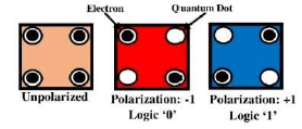
Previously, complementary metal-oxide-semiconductor (CMOS) technology was the dominant technique for designing nano-scale electronic circuits. Many problems plagued CMOS technology and the fact that it is rapidly reaching its physical boundaries [1]. Then emerged a slew of alternative technologies, with Quantum-dot Cellular Automata (QCA) being one of the most promising for resolving these challenges and continuing nano-level design. This concept was first proposed by C. S. Lent et al. in 1993 for nano-level circuit design [1]. This method is essentially based on the tunneling of electrons within a square shaped semiconductor cell known as a QCA cell, which has four quantum dots at each corner [2]. As a result, a cell, as shown in Fig. 1, is the smallest unit of QCA technology. Due to Coulombic repulsive force, two electrons can travel within the cell among the four dots and try to pick the diagonal locations of the square, which is the largest distance between them [1]. As a result, two configurations are available, as indicated in Fig. 1: polarisation ‘-1’ or logic 0 and polarisation ‘+1’ or logic 1 [2]. In 1997, the notion of QCA cell manufacture was developed [3].
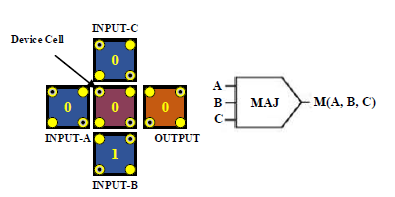
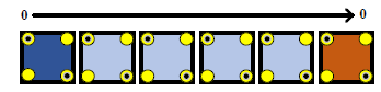
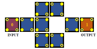
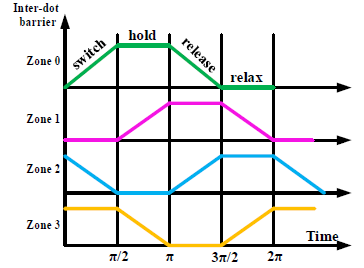
The majority gate or majority voters, QCA-wire, and QCA-inverter, are the core elements of QCA technology, and these elements may be used to build different logic circuits. A majority voter has three inputs and one output, as shown in Fig. 2 [4]. The majority voter’s driver cell is that cell located at the center. It behaves as an AND gate if one of the three inputs is fixed at polarization ‘-1’, and as an OR gate if one of the three inputs is fixed at polarization ‘+1’, [4]. As seen in Fig. 2, the output follows the equation AB + BC + CA for three inputs A, B, and C. The arrangement of a few cells in a series called QCA wire, as illustrated in Fig. 3, is in which the input polarization is transferred from one cell to the next until it reaches the output without making any changes [5]. When two cells are positioned diagonally, as illustrated in Fig. 4, it operates as a NOT gate, which is known as a QCA inverter [4]. There is no requirement for an additional bias voltage source; instead of, QCA may conduct operations by utilizing the four clocks internally, and there is a 90-degree phase difference between each phase of the four clocks to ensure low power depletion [5]. Each clock has four stages: the switch phase, hold phase, release phase, and relax phase, as shown in Fig. 5 [6].
Basically, the extensive research work in the QCA domain has yet to be completed in terms of designing and modeling of digital circuits. Researchers have already been described components used for the designing and modeling of digital circuits such as Logic gates [7, 8], adders [9, 10], subtractors [11, 12], comparator [13], multiplier [14], flip-flops and memory [15, 16], registers [17-19], counters [20, 21], arithmetic logic units (ALU) [22, 23], etc. Researchers have recently focused on the field of nano communication. Multiplexer and demultiplexer circuits have been chosen as the essential design elements because they are simple and have several uses in the field of nano communication. In this article, a simple and basic multiplexer and demultiplexer are considered experimental objects. The projected multiplexer and demultiplexer designs are motivated by the work reported in [24] and [25]. It should be noted that both the experimental entities, namely multiplexer, and demultiplexer, are relatively simple in that they occupy a small amount of area and have a low level of cell complexity. The estimation of energy loss and simple circuits costs are contemporary QCA technological advances that have accelerated our study. Simple QCA multiplexer and demultiplexer design is important and have their assigned applications in the field of nano communication and nano computation, such as nano switch, reversible computing circuits, nano router, and so on. In QCA technology, the modern and advanced design trends are given as follows:
Figure 1. QCA cell
Figure 2. QCA Majority voters or Majority gate
Figure 3. QCA Wire
Figure 4. QCA Inverters
Figure 5. QCA clocking scheme
Multiplexers and demultiplexers have clogged the QCA literature. Over the past few years, there have been several good designs have been made that have been discussed. Roohi et al. (2011) created a 2:1 multiplexer with a complexity of twenty-seven clocks [26]. Kianpour et al. (2013) proposed a simple and basic multiplexer design that contains twenty-two cells and three clocks [27], whereas Chabi et al. (2014) extended a multiplexer almost identical to the previous designs, which includes twenty-three cells and three number of clock zones similar to the previous design [28]. Likewise, B. Sen et al. (2015) constructed an efficient 2:1 multiplexer with only two clocks employing twenty-three cells [29]. Rashidi et al. (2016) devised a multiplexer that consists of fifteen-cell with an area of each cell is 0.01 µm2 [30]. J. C. Das et al. (2016) created a 2:1 multiplexer with the help of three majority voters and one inverter. It is found that the area has been utilized by 47.22% [31]. Rashidi et al. (2017) developed the multiplexer layout with the help of basic gates such as two AND gates, one OR gate, and one NOT gate [32]. Asfestani et al. (2017) developed an efficient and cost-effective QCA multiplexer structure without any help from the majority voter [33]. Khosroshahy et al. (2017) investigated a different method for minimizing the multiple inputs fed in multiplexers externally [34]. F. Ahmad (2017) proposed a procedure to design a 2n: 1 QCA multiplexer, whereas Ahmadpour et al. (2018) constructed a fault-tolerant multiplexer in QCA technology by utilizing the four clocks and used the QCAPro tool to estimate the energy loss with complexity 36 [35, 36]. M. Mosleh (2018) discussed a multilayer design approach by utilizing the new majority voter (MV32) idea [37]. L Xingjun et al. (2019) investigated a 2:1 multiplexer by utilizing 22 cells with an overall area of 0.03 µm2 [38]. E. AlKaldy et al. (2020) developed an optimum design of a QCA multiplexer by utilizing the 11 cells without requiring any majority voters [39]. In the same way, there are various examples in the literature to design QCA multiplexers, which might make this topic extremely lengthy. The QCA demultiplexer unit, however, is an exception. In the QCA literature, despite the intensification of multiplexers, it lacks contributions to demultiplexer design. To maintain the continuity of the discussion, a couple of decent demultiplexers we’re discussing here. For designing the circuit in the highest order, N. A. Shah et al. (2011) proposed a modular demultiplexer with the help of 56 cells [40]. J. Iqbal et al. (2013) proposed another modular 1:2 demultiplexer with complexity 27 [41]. L. H. B. Sardinha et al. (2015) developed a nano communication demultiplexer [42]. N. Safoev et al. (2016) presented a multilayer 1:2 demultiplexer structure with a couple of clocks and 21 cells [43]. F. Ahmad (2017) recommended a demultiplexer with 21 cells, while J. C. Das et al. (2017) suggested a demultiplexer with 32 cells [35, 44]. Apart from the above list of QCA demultiplexers, no other demultiplexer designs are known to have existed in the literature. Nevertheless, the number of articles never exceeds the number of QCA multiplexer research. As a result, the following are the significant gaps in the QCA literature:
From the literature, the aforementioned gaps have been identified and addressed by examining a basic multiplexer and a simple demultiplexer in this study. The layouts were designed using the QCADesigner-2.0.3 [45] simulation environment. $\mathrm{QCADe}$ igner- $\mathrm{E}(\mathrm{QDE})[46]$ tool used the Range-Kutta method is used for the approximation and estimate of the energy in the Coherence vector mode. In addition, a separate tool, QCAPro [47], was utilized to calculate energy dissipation, making this paper more robust. Different cost-effective functions and other design characteristics have been introduced for better analysis.
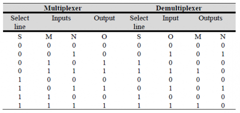
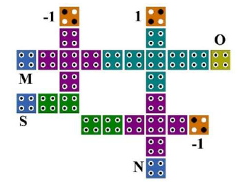
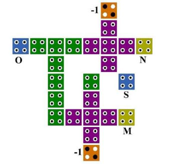
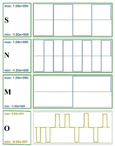
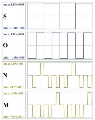
In this article, a QCA multiplexer (MUX) and a QCA demultiplexer (DEMUX) are the experimental entities. By employing the QCA technique, the design of layouts of both units is pretty straightforward. The proposed QCA layout of a basic 2:1 MUX is illustrated in Fig. 6. It consists of two input lines represented as ‘M’ and ‘N’, one select line is represented as ‘S’, and one output line denoted as ‘O’. From Fig. 7, the proposed QCA layout of a simple 1:2 DEMUX consists of one input line denoted as ‘O’, one select line is represented as ‘S’, and two output lines represented as ‘M’ and ‘N’, respectively. The appropriate truth table for the proposed QCA MUX and QCA DEMUX is given in Table 1. Simulation results of the proposed QCA MUX and DEMUX are demonstrated in Fig. 8 and Fig. 9, respectively.
The proposed QCA MUX has a complexity of 28 with a cell area consisting of 9072 nm2= 0.009072 µm2and a total area of 54102 nm2 = 0.05 µm2. In contrast, the proposed QCA DEMUX has a complexity of 24 with a cell area consisting of 7776 nm2= 0.007776 µm2 and a total area of 44719 nm2 = 0.04 µm2.
Table 1. Logic table of multiplexer and demultiplexer
All the essential QCA-layout design matrices have been discussed below for the proposed multiplexer and demultiplexer:
Complexity
The complexity is defined as the total number of cells required to build a QCA layout. The suggested 2:1 QCA MUX requires 28 cells with a complexity of 28, while the proposed 1:2 QCA DEMUX with a complexity of 24.
Occupied Area
In QCA designs, there are two area parameters: cell area and total area. Cell area is the region used by the design’s cells, and it's computed by multiplying cell count by $(18 \times 18) \mathrm{nm}^{2}$. This proposed multiplexer has a cell area requirement of 9072 $\mathrm{nm}^{2}=0.009072 \mathrm{\mu m}^{2}$ and a total area requirement of $54102 \mathrm{~nm}^{2}$ $=0.05{\mu \mathrm{m}^{2}}^{2}$. In contrast, the proposed demultiplexer has a cell area requirement of $7776 \mathrm{~nm}^{2}=0.007776 \mathrm{um}^{2}$, and a total area requirement of $44719 \mathrm{~nm}^{2}=0.04 \mu \mathrm{m}^{2}$.
Area usage
We know that the following equation would be used to indicate the percent of area usage:
area usage $=\frac{\text { cell area needed }}{\text { total area needed }} \times 100 \%$
The area of utilization of the projected multiplexer is evaluated as 16.76%, and the utilized area of the demultiplexer is evaluated as 17.39%.
Figure 6. Proposed QCA multiplexer unit
Figure 7. Proposed QCA demultiplexer unit
Number of clock phases used
For the successful simulation of the proposed QCA MUX and QCA DEMUX, there is three and two clock phases or clock zones are used.
Latency in clock-cycle
The time difference between the output and the input is called latency in the clock-cycle. It is also known to be the input-to-output latency. The suggested multiplexer has a delay of 0.75-clock-cycle since it uses 3-clock-phases in the worst path to reach output from input. We know that four clock phases equal a 1-clock-cycle. Similarly, the latency of the proposed demultiplexer is 0.5-clock-cycle.
Number of used gates
There is only a single inverter, and three majority voters (majority gates) have been used to construct the proposed QCA MUX, respectively. In the case of QCA DEMUX, there are a couple of inverters and one majority gate has been used, respectively.
Number of used crossovers
No wire-crossing has been used to design the QCA layout for both the experimental items. In addition, both the layouts are single-layered.
Energy estimate is a new trend in QCA circuit analysis. QCAPro tool is a standard tool used to estimate the energy and also the cell to cell energy dissipation calculation. QCAPro tool is the most commonly used energy computation tool, which is very well known. Unfortunately, it won’t be worked with any newer or advanced versions of tools, like QCADesigner-2.0.3. QCAPro only supports older versions of the tool, QCADesigner-1.0.0, and QCADesigner-1.0.1. It is the shortcomings of this tool.
However, QCADesigner-E (or QDE) is a relatively advanced tool that is used for the coordinate-based estimation of energy dissipation of the multiplexer and demultiplexer. One of the two approximation-based approaches (that is, the Eular technique or the Range-Kutta approach) is required to evaluate the energy loss (or energy dissipation) using QDE. In the previous work, authors in [25], [48] evaluated the energy with the help of the Euler approach. However, the same is presented here using the Range-Kutta approximation approach.
Figure 8. Simulation output of QCA multiplexer
Figure 9. Simulation output of QCA demultiplexer
A brief discussion about QCAPro is required to preserve the continuation. We may estimate the non-adiabatic energy loss of QCA logic circuits using the QCAPro tool. Its foundation is the well-known Hartree-Fock approximation [49, 50]. By using the Hamiltonian matrix [47], the overall energy of the QCA cell has been computed, which reflects the Colubmic interaction between cells and is indicated in equation (1).
$\widehat{H}_{l}=\left[\begin{array}{cc}\frac{-E_{k}}{2} \sum_{i} C_{j} f_{i, j} & -\gamma \\ -\gamma & \frac{+E_{k}}{2} \sum_{i} C_{j} f_{i, j}\end{array}\right]$ (1)
where $C_{i}$ represents the polarization of $i^{t h}$ adjacent cell, the geometrical factor which is related to the electrostatic interaction between $i^{\text {th }}$ cell and $j^{\text {th }}$ cell is denoted by $f_{i, j}$, and the tunneling energy between two cell states is represented by $\gamma[49,50]$. The anticipated energy value of a cell for every clock cycle is derived and expressed as in equation (2).
$E=\langle H\rangle=\frac{\hbar}{2} \times \Gamma \times \lambda$ (2)
During the estimation of energy loss by using the QDE tool, the expression of the instantaneous power flow into a QCA cell can be written as
$P_{t o}=\frac{d E}{d t}=\frac{\hbar}{2}\left[\frac{d \Gamma}{d t} \cdot \lambda\right]+\frac{\hbar}{2}\left[\Gamma \cdot \frac{d \lambda}{d t}\right]$ (3)
where $\lambda$ denotes the coherence vector, the $3-\mathrm{D}$ (threedimensional) energy vector is represented by $\Gamma$, and the reduced Planck constant denoted by $\hbar$.
In equation (3), the first part of instantaneous power is $\frac{\hbar}{2}\left[\frac{d \Gamma}{d t} \cdot \lambda\right]$, which combines the cell-to-cell power and clock inout power [50]. The second part of the instantaneous power is $\frac{\hbar}{2}\left[\Gamma \cdot \frac{d \lambda}{d t}\right]$ which combines the instantaneous power itself and dissipated power $[50]$. For a given period of time $[-\mathrm{T},+\mathrm{T}]$, the energy dissipated from a QCA cell is given as
$E_{d}=\frac{\hbar}{2} \int_{-T}^{+T}\left[\Gamma \cdot \frac{d \lambda}{d t}\right] d t$ (4)
Similarly, we can determine the leakage power loss (energy dissipation) and switching power loss with the help of equation (5) and equation (6), respectively [50].
$P_{\text {leakage }}=\frac{1}{2^{r}} \sum_{i=1}^{N-r} P_{i, n \rightarrow m}^{\text {leakage }}$ (5)
$P_{\text {switch }}=\frac{1}{2^{r}} \sum_{i=1}^{N-r} P_{i, n \rightarrow m}^{\text {switch }}$ (6)
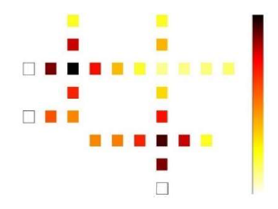
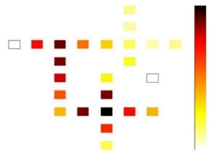
The energy dissipation may be measured in three tunneling energy levels with $\gamma=0.5 \mathrm{E}_{\mathrm{K}}, \gamma=1.0 \mathrm{E}_{\mathrm{K}}$, and $\gamma=1.5 \mathrm{E}_{\mathrm{K}}$ at a fixed temperature $(2 \mathrm{~K})$ using the tool QCAPro. We can find out the energy loss due to leakage, switching, and the overall loss with the help of the QCAPro tool. According to the QCAPro tool, the aggregate energy dissipation of the proposed QCA multiplexer is $35.60$ meV at $\gamma=0.5 \mathrm{E}_{\mathrm{K}}$, is $48.39$ meV at $\gamma$ $=1.0 \mathrm{E}_{\mathrm{K}}$ and is $63.71 \mathrm{meV}$ at $\gamma=1.5 \mathrm{E}_{\mathrm{K}}$. The aggregate energy dissipation of the proposed demultiplexer is $37.19$ meV at $\gamma=$ $0.5 \mathrm{E}_{\mathrm{K}}$, is $47.63 \mathrm{meV}$ at $\gamma=1.0 \mathrm{E}_{\mathrm{K}}$ and is $60.34 \mathrm{meV}$ at $\gamma=0.5$ $\mathrm{E}_{\mathrm{K}}$. Fig. 10 and Fig. 11 illustrates the polarization hotspots of the proposed multiplexer and demultiplexer, as measured using QCAPro at $\gamma=0.5 \mathrm{E}_{\mathrm{K}}$ and $2 \mathrm{~K}$ temperatures, respectively. Using QCAPro $\gamma=0.5 \mathrm{E}_{\mathrm{K}}$ and $2 \mathrm{~K}$ temperature, the energy hotspots of the multiplexer are displayed in Fig. 12, and the same for the demultiplexer is presented in Fig. 13. The deeper colors denoted higher energy dissipation and polarization levels. Table 2 depicts the energy dissipation of the proposed items using QCAPro.
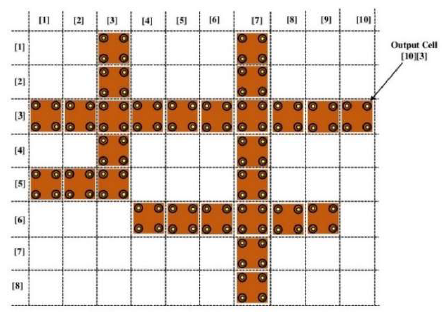
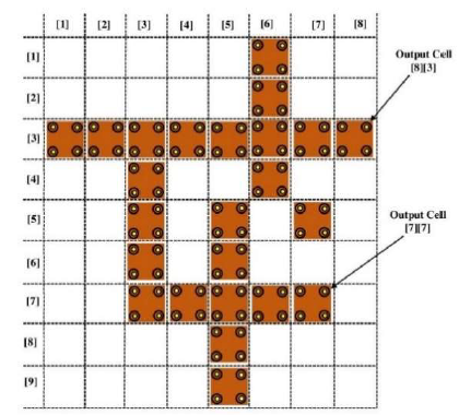
QCADesigner-E or QDE is a new tool for energy estimation, which is an extension of the popular tool QCADesigner. We calculated the energy dissipation based on the Runge Kutta approximation [46]. In a QCA cell, an array of the cell is considered and assigns coordinate numbers to each individual cell. For the mathematical analysis of QCADesigner, the cell can be treated as a bath of energies (that is, soaking of energy) [46]. Let E_BATH represent the overall amount of energy that gets transferred and separated from the respective clock cycle to the ‘bath’ of all QCA cells, and the overall energy loss is given as $\sum_{\text {all }} E_{2} B A T H[52,53]$. The three components of energy loss have been added to determine the overall energy loss, and it is given as $\sum_{\text {all }} E_{-} B A T H=E_{C K}+E_{E V}+E_{I O}$, where $E_{\mathrm{CK}}$ denotes the aggregate of all the energy between QCA cells, and the clock gets transferred and separated by each clock cycle, $E_{E V}$ represents the energy that transfers between the QCA cells and the environment, and $E_{\text {IO }}$ denotes the movement of energy transferred amongst QCA cells [46]. Note that $\mathrm{E}_{\mathrm{IO}}=\mathrm{E}_{\mathrm{IN}}-\mathrm{E}_{\text {OUT }}$ for $\mathrm{QCA}$ wire, where $\mathrm{E}_{\mathrm{IN}}$ denotes the energy that gets entered inside the QCA cell, and EouT represents the energy left from the QCA cell. During the evaluation of loss of energy, a minor mistake may occur is represented as $\mathrm{E}_{\mathrm{RR}}$. The overall analysis of QCA cell energy errors for each clock cycle is expressed as $E_{R R}=E_{\mathrm{EV}}-\left(E_{C K}+\right.$ $\mathrm{E}_{\mathrm{IO}}$ ) [46]. Depending on the transmission of energy direction, an error can be either '+' or '-'. If the error is '+', the positive energy value has been transferred and transported to the nearby environments to $\mathrm{E}_{\mathrm{EV}}, \mathrm{E}_{\mathrm{IO}}$, and $\mathrm{E}_{\mathrm{CK}}$. The energy was estimated using the Runge Kutta approximation and 'array coordinates' as presented by QDE [46]. '[column number] [row number]' is the format for the array coordinates. A total of 500000 samples were taken and examined for the simulation with coherence vector energy as the simulation mode. The QCA multiplexer's overall energy loss is $14.30$ $m e V$, with a minor error of $-1.41 m e V$, and its average energy loss per cycle is $1.30 \mathrm{meV}$, with a negligible error of $-0.128$ $m e V$. Similarly, the demultiplexer has an aggregate energy consumption of $7.37 \mathrm{meV}$ with a trivial error of $-0.654 \mathrm{meV}$, and the average energy loss per cycle is $0.670 \mathrm{meV}$ with a negligible error of $-0.0595 \mathrm{meV}$. Fig. 14 and Fig. 15 illustrate the 'array coordinates' of the multiplexer and demultiplexer, respectively. Table 3 and Table 4 show the energy dissipation values in meV of the multiplexer's output coordinates '[10] [3]' and the demultiplexer's one output coordinates ' $[8][3]$ '.
During the evaluation of the performance of a QCA circuit, the cost is an essential parameter or element which needs to be considered. Cost is also one of the most important research trends currently in QCA circuit design, which is used to assess the cost for better performance analysis.
6.1 Area-delay Cost
Area-delay cost is defined as the generic cost of QCA circuits. It is considered as the performance metric mostly used for circuit performance analysis, where most researchers are looking to improve performance. It can be figured out by utilizing the overall area to build the QCA architecture as well as by using the input to output delay. Input to output delay is now called as latency, where the output delay is relatively dependent to the input. The number of clock-cycle has been used to represent the latency or delay. Our experimental MUX and DEMUX have the same delay, which is 0.5-clock-cycle, or half a clock-cycle. The relation between area and delay cost can be expressed as (Area) × (latency)2[51, 52]. The overall area and latency for the proposed QCA MUX are 0.05 μm2and 0.75-clock-cycle, respectively. Then, the area-delay cost for the proposed QCA MUX is evaluated as 0.028125 μm2-(clock- cycle)2. Similarly, for the proposed QCA DEMUX, the overall area and latency are 0.04 μm2and 0.5-clock-cycle, respectively. Then, the area-delay cost for the proposed QCA DEMUX is evaluated as 0.01 μm2-(clock-cycle)2.
6.2 QCA-specific Cost
This parameter is mainly considered for the QCA circuits. Also called it as figure of Merit (FoM) given by $[51,52]$. The number of employed majority voters (MV), clocks (CK), crossover (CV), and inverters is taken into consideration to make a QCA architecture. The evaluation of QCA-specific cost for QCA circuits can be expressed as FoM is $\left(\left(M V^{m}+I N\right.\right.$ $\left.\left.+C V^{m}\right) \times C K^{p}\right)[50,54]$. Where $m, n$, and $p$ represent the majority voter, crossover, and clocks count of experimental loads. Commonly, the value of weights will be considered $m$ $=n=p=2$ as fixed value $[50,54]$. For the proposed $\mathrm{QCA}$ MUX, the FOM is calculated as $\left(3^{2}+1+0\right) \times 3^{2}=90$ and the FOM for the proposed QCA DEMUX is reported as $\left(2^{2}+2+\right.$ $0) \times 2^{2}=24$.
Figure 10. Polarization hotspots of the proposed multiplexer
Figure 11. Polarization hotspots of the proposed demultiplexer
Figure 12. Energy hotspots of proposed multiplexer
Figure 13. Energy hotspots of the proposed demultiplexer
6.3 Energy-delay Cost
The energy dissipations were computed using the QDE and QCAPro tools, resulting in two different energy-delay cost functions. However, using the QCAPro tool, in this study, theenergy-latency cost will be determined exclusively by assessing the energy losses (meV) at the 1.0EK tunneling energy level. It’s very valuable to note that the evaluation may be the same for tunneling energy levels 0.5EK and 1.5EK as well. The formulation for the calculation of the parameter called energy-latency cost is expressed as (Ex × Dy), where E denotes the loss of energy, D represents the latency (or delay), $x=y$ depicts the experimental loads (weights) $[51,52]$. The generic value of experimental loads will be considered as $2(x$ $=y=2)$ for the present experiment. The overall energy loss will be evaluated for the proposed QCA MUX, and QCA DEMUX at temperature $2 \mathrm{~K}$ with $1.0 \mathrm{E}_{\mathrm{K}}$ tunneling energy levels is $48.39 \mathrm{meV}$ and $47.63 \mathrm{meV}$, respectively. For the proposed QCA MUX and QCA DEMUX, the latency is evaluated as $0.75$-clock-cycle and 0.5-clock-cycle, respectively. Therefore, the energy-latency cost for the proposed QCA MUX is calculated as $(48.39)^{2} \times(0.75)^{2}=$ $1317.145556$ meV$^{2}$-(clock-cycle) ${ }^{2}$. Similarly, the energylatency cost for the proposed QCA DEMUX is calculated as $(47.63)^{2} \times(0.5)^{2}=567.154225$ meV $^{2}-(\text { clock-cycle })^{2}$.
Figure 14. Array coordinates of QCA multiplexer in QDE
Figure 15. Array coordinates of QCA demultiplexer in QDE
From the last five years of literature on QCA circuit design, this article has selected some well and accurate designs of QCA for comparison. To make a comparison, this article considers one of the most important parameters, which is energy loss computation. Nevertheless, in recent research, the energy loss parameter by multiplexer or demultiplexer has not been taken into consideration. Only E. Alkaldy et al. (2020) [36] and F. Ahmad (2017) [35] utilized the tool called QCAPro tool to determine the energy loss by multiplexer. Even so, there is no work to be done included previously for the evaluation of energy loss by the demultiplexer. However, this work used the Range Kutta approximation in the QDE tool to dissipate energy. Also, QCAPro-based energy dissipation has been discussed. It is one of the most significant benefits of this work.
Consideration of cost functions will be the other most prominent factor. This parameter has been discussed in a broad manner. This work has been examined in three types of cost functions, but there is no work that has been done and addressed the issues previously. The area-delay cost for the proposed QCA MUX and QCA DEMUX are properly designed since their area-latency (or delay) cost is 0.028125- unit and 0.01-unit, respectively. In the same way, the presented multiplexer and demultiplexer have computed QCA-specific costs or FoMs of 90 and 24, respectively, which are acceptable values. The proposed QCA MUX and QCA DEMUX have calculated energy-latency costs of 1317.145556-unit and 567.154225-unit, respectively. It’s very important to note that there is no research work done to estimate all the cost parameters for the proposed QCA MUX and DEMUX. Table 5 and Table 6 include a few general metrics such as complexity, area, area utilization, counting clocks, latency (or delay), and gate count of multiplexer and demultiplexer, respectively, to help comparisons.
The experiment used QCA architectures with minimal circuit complexity, area demand, and cost. They have lower energy dissipation, as determined by QDE calculations. In an experimental examination of energy estimates utilizing QCADesigner-E or QDE, low energy losses were discovered for both circuits. In the present era of QCA technology trends, this article is very valuable because it perfectly follows the current design trends. In this article, an evaluation of three different sorts of costs has been done. Here, we address the basic MUX and simple DEMUX area-latency, QCA-specific, and energy-latency costs to show that the objects are more than efficient.
As an outcome of this work, these small blocks construct a method for designing higher-order nano computational circuits, particularly nano-communication devices such as nano-routers, in which MUX and DEMUX are inescapable blocks. This part should include the research’s primary findings as well as a clear explanation of their significance and relevance. It is also possible to discuss the work’s weaknesses and potential research directions.
Table 2. Energy losses of proposed modules using QCAPro
|
Circuits |
Leakage energy loss (meV) |
Switching energy loss (meV) |
Total energy loss (meV) |
||||||
|
|
0.5EK |
1.0EK |
1.5EK |
0.5EK |
1.0EK |
1.5EK |
0.5EK |
1.0EK |
1.5EK |
|
MUX |
9.23 |
26.01 |
44.83 |
26.37 |
22.38 |
18.88 |
35.60 |
48.39 |
63.71 |
|
DeMUX |
6.87 |
20.64 |
36.86 |
30.32 |
26.99 |
23.48 |
37.19 |
47.63 |
60.34 |
Table 3. Energy loss (meV) of the output coordinates [10][3] of multiplexer using QDE
|
EBATH |
ECK |
EIO |
EIN |
EOUT |
ERR |
EK |
EBATH_total |
ECK_total |
ERR_total |
|
0.017557 |
-0.0076949 |
-0.011224 |
-0.011224 |
0.0000 |
-0.0013615 |
EK [0] =+1.48361100 |
1.7615 |
0.050822 |
-0.17972 |
|
0.017523 |
-0.0076849 |
-0.011196 |
-0.011196 |
0.0000 |
-0.0013578 |
EK [1] = -0.00197461 |
1.2447 |
0.92239 |
-0.12145 |
|
0.010213 |
-0.0063277 |
-0.0044324 |
-0.0044324 |
0.0000 |
-0.00054687 |
EK [2] = +0.00092847 |
0.61699 |
1.5635 |
-0.052036 |
|
0.017558 |
-0.0076941 |
-0.011226 |
-0.011226 |
0.0000 |
-0.0013616 |
EK [3] = +0.04413817 |
1.7710 |
0.15963 |
-0.18139 |
|
0.010292 |
-0.0016754 |
0.0059024 |
0.0059024 |
0.0000 |
-0.00055968 |
EK [4] = +0.00092847 |
1.7075 |
0.13696 |
-0.17396 |
|
0.010296 |
-0.0016795 |
0.0059390 |
0.0059390 |
0.0000 |
-0.00056015 |
EK [5] = -0.001974610 |
1.1908 |
1.0088 |
-0.11568 |
|
0.010208 |
-0.0063252 |
-0.0044289 |
-0.0044289 |
0.0000 |
-0.00054632 |
EK [6] = +0.00092847 |
1.2311 |
0.69247 |
-0.12123 |
|
0.017555 |
-0.0076805 |
-0.011235 |
-0.011235 |
0.0000 |
-0.0013612 |
EK [7] = -0.001974610 |
1.1564 |
1.0321 |
-0.11284 |
|
0.017557 |
-0.0076949 |
-0.011224 |
-0.011224 |
0.0000 |
-0.0013615 |
EK [8] = +0.00572710 |
1.7615 |
0.050822 |
-0.17972 |
|
0.017523 |
-0.0076849 |
-0.011196 |
-0.011196 |
0.0000 |
-0.0013578 |
|
1.2447 |
0.92239 |
-0.12145 |
|
0.010213 |
-0.0063277 |
-0.0044324 |
-0.0044324 |
0.0000 |
-0.00054687 |
|
0.61699 |
1.5635 |
-0.052036 |
Table 4. Energy loss (meV) of one of the output coordinates [8][3] of demultiplexer using QDE
|
EBATH |
ECK |
EIO |
EIN |
EOUT |
ERR |
EK |
EBATH_total |
ECK_total |
ERR_total |
|
0.0090578 |
0.0019017 |
-0.011395 |
-0.011395 |
0.0000 |
-0.00043584 |
EK[0] = -0.001974610 |
0.41713 |
0.29614 |
-0.030987 |
|
0.0099539 |
-0.031252 |
0.020750 |
0.020750 |
0.0000 |
-0.00054837 |
EK [1] = +0.00148361 |
1.0672 |
-0.20694 |
-0.10404 |
|
0.0090143 |
-0.0032474 |
-0.0061998 |
-0.0061998 |
0.0000 |
-0.00043299 |
EK [2] = -0.009219376 |
0.43238 |
0.51618 |
-0.032656 |
|
0.036771 |
0.0034155 |
-0.043684 |
-0.043684 |
0.0000 |
-0.0034978 |
EK [3] = -0.01021058 |
0.80964 |
0.088890 |
-0.075597 |
|
0.0090578 |
0.0019017 |
-0.011395 |
-0.011395 |
0.0000 |
-0.00043584 |
EK [4] = -0.01021058 |
0.41713 |
0.29614 |
-0.030987 |
|
0.0099539 |
-0.031252 |
0.020750 |
0.020750 |
0.0000 |
-0.00054837 |
EK [5] = -0.01021058 |
1.0672 |
-0.20694 |
-0.10404 |
|
0.0090143 |
-0.0032474 |
-0.0061998 |
-0.0061998 |
0.0000 |
-0.00043299 |
EK [6] = +0.04413817 |
0.43238 |
0.51618 |
-0.032656 |
|
0.036771 |
0.0034155 |
-0.043684 |
-0.043684 |
0.0000 |
-0.0034978 |
EK [7] = +0.00572710 |
0.80964 |
0.088890 |
-0.075597 |
|
0.0090578 |
0.0019017 |
-0.011395 |
-0.011395 |
0.0000 |
-0.00043584 |
|
0.41713 |
0.29614 |
-0.030987 |
|
0.0099539 |
-0.031252 |
0.020750 |
0.020750 |
0.0000 |
-0.00054837 |
|
1.0672 |
-0.20694 |
-0.010404 |
|
0.0090143 |
-0.0032474 |
-0.0061998 |
-0.0061998 |
0.0000 |
-0.0004329 |
|
0.43238 |
0.51618 |
-0.032656 |
Table 5. Comparative analysis of proposed multiplexer with prior reported works
|
2: 1 MUX |
COM |
CA (μm2) |
TA (μm2) |
AU (%) |
#CU |
LAT (CL) |
#CRV |
|
Ref. [24] |
17 |
0.005508 |
0.01 |
55.08 |
3 |
0.75 |
0 |
|
Ref. [30] |
15 |
0.00486 |
0.01 |
48.60 |
2 |
0.5 |
0 |
|
Ref. [31] |
17 |
0.005508 |
0.011664 |
47.22 |
3 |
0.75 |
0 |
|
Ref. [32] |
17 |
0.005508 |
0.02 |
27.54 |
2 |
0.5 |
0 |
|
Ref. [33] |
12 |
0.003888 |
0.01 |
38.88 |
1 |
0.25 |
0 |
|
Ref. [34] |
42 |
0.013608 |
0.04 |
34.02 |
4 |
1 |
0 |
|
Ref. [35] |
16 |
0.005184 |
0.01 |
51.84 |
2 |
0.5 |
0 |
|
Ref. [36] |
35 |
0.011340 |
0.04 |
28.35 |
4 |
1 |
0 |
|
Ref. [37] |
21 |
0.006804 |
0.01 |
64.04 |
3 |
0.75 |
3 |
|
Ref. [38] |
22 |
0.007128 |
0.03 |
23.76 |
3 |
0.75 |
0 |
|
Ref. [39] |
11 |
0.003564 |
0.01 |
35.64 |
1 |
0.25 |
0 |
|
PM |
17 |
0.009072 |
0.05 |
18.144 |
3 |
0.75 |
0 |
|
2: 1 MUX |
#MG |
#NOT |
ADC |
QSC |
EA |
ED (meV) |
EDC |
|
Ref. [24] |
3 |
1 |
0.005625 |
90 |
No |
NA |
NA |
|
Ref. [30] |
3 |
1 |
0.0025 |
40 |
No |
NA |
NA |
|
Ref. [31] |
3 |
1 |
0.00656 |
90 |
No |
NA |
NA |
|
Ref. [32] |
3 |
1 |
0.005 |
40 |
No |
NA |
NA |
|
Ref. [33] |
1 |
0 |
0.000625 |
1 |
No |
NA |
NA |
|
Ref. [34] |
3 |
3 |
0.04 |
192 |
No |
NA |
NA |
|
Ref. [35] |
2 |
1 |
0.0025 |
20 |
QCAPro |
21.82 |
109 |
|
Ref. [36] |
3 |
1 |
0.04 |
160 |
No |
NA |
NA |
|
Ref. [37] |
3 |
1 |
0.005625 |
171 |
No |
NA |
NA |
|
Ref. [38] |
2 |
1 |
0.016875 |
45 |
No |
NA |
NA |
|
Ref. [39] |
1 |
0 |
0.000625 |
1 |
QCAPro |
17.62 |
20 |
|
PM |
3 |
1 |
0.028125 |
90 |
QCAPro, QDE |
48.39 |
1317 |
*PM: Proposed multiplexer, COM: Complexity, CA: Cell area, TA: Total area, AU: Area usage, #CU: Number of clocks used, LAT (CL): Latency (in clock-cycle), \#CRV: Number of crossovers used, #MV: Number of majority voters used, #NOT: Number of inverters used, ADC: Area-delay cost in $\mu m^{2}$-(clock-cycle) , QSC: QCA specific cost, EA: Energy analysis, ED: Energy loss at $\gamma=1.0 \mathrm{E}_{\mathrm{K}}$ in $m e V$, EDC: energy-delay cost in meV²-(clock-cycle) ${ }^{2}$.
Table 6. Comparative analysis of proposed demultiplexer with prior reported works
|
1: 2 DeMUX |
COM |
CA (μm2) |
TA (μm2) |
AU (%) |
#CU |
LAT (CL) |
#CRV |
|
Ref. [35] |
21 |
0.006804 |
0.03 |
34.02 |
2 |
0.5 |
0 |
|
Ref. [43] |
21 |
0.006804 |
0.01 |
68.04 |
2 |
0.5 |
0 |
|
Ref. [44] |
32 |
0.010368 |
0.02 |
51.84 |
3 |
0.75 |
1 |
|
PD |
24 |
0.007776 |
0.04 |
19.44 |
2 |
0.5 |
0 |
|
1: 2 DeMUX |
#MG |
#NOT |
ADC |
QSC |
EA |
ED (meV) |
EDC |
|
Ref. [35] |
2 |
1 |
0.0075 |
20 |
No |
NA |
NA |
|
Ref. [43] |
2 |
1 |
0.0025 |
20 |
No |
NA |
NA |
|
Ref. [44] |
2 |
1 |
0.01125 |
54 |
No |
NA |
NA |
|
PD |
2 |
2 |
0.01 |
24 |
QCAPro, QDE |
47.63 |
3.6298 |
*PD: Proposed demultiplexer, COM: Complexity, CA: Cell area, TA: Total area, AU: Area usage, #CU: Number of clocks used, LAT (CL): Latency (in clockcycle), #CRV: Number of crossovers used, #MV: Number of majority voters used, #NOT: Number of inverters used, ADC: Area-delay cost in $\mu m^{2}$ - (clock-cycle) $)^{2}$, QSC: QCA specific cost, EA: Energy analysis, ED: Energy loss at $\gamma=1.0 \mathrm{E}_{\mathrm{K}}$ in $m e V$, EDC: energy-delay cost in $m e V^{2}-(c l o c k-c y c l e)^{2}$.
[1] Lent, C. S., Tougaw, P. D., Porod, W., Bernstein, G. H. (1993). Quantum cellular automata. Nanotechnology, 4(1): 49-57. https://doi.org/10.1088/0957-4484/4/1/004.
[2] Orlov, A. O., Amlani, I., Bernstein, G. H., Lent, C. S., Snider, G. L. (1997). Realization of a functional cell for quantum-dot cellular automata. Science, 277(5328): 928- 930. https://doi.org/10.1126/science.277.5328.928.
[3] Lent, C. S., Tougaw, P. D. (1997). A device architecture for computing with quantum dots. Proceedings of the IEEE, 85(4): 541-557. https://doi.org/10.1109/5.573740.
[4] Tougaw, P.D., Lent, C.S. (1994). Logical devices implemented using quantum cellular automata. Journal of Applied Physics, 75(3): 1818–1825. https://doi.org/10.1063/1.356375.
[5] Lent, C.S., Tougaw, P.D. (1993). Lines of interacting quantum-dot cells: a binary wire. Journal of Applied Physics, 74(10): 6227–6233. https://doi.org/10.1063/1.355196.
[6] Tóth, G., Lent, C. S. (1999). Quasiadiabatic switching for metal-island quantum-dot cellular automata. Journal of Applied Physics, 85(5): 2977–2984. https://doi.org/10.1063/1.369063.
[7] Kavitha, S. S., Kaulgud, N. (2017). Quantum dot cellular automata (qca) design for the realization of basic logic gates. 2017 International Conference on Electrical, Electronics, Communication, Computer, and Optimization Techniques (ICEECCOT), Mysuru, 2017, pp. 314-317. https://doi.org/10.1109/ICEECCOT.2017.8284519.
[8] Balakrishnan, L., Godhavari, T., Kesavan, S. (2015). Effective design of logic gates and circuit using quantum cellular automata (qca). 2015 International Conference on Advances in Computing, Communications and Informatics (ICACCI), Kochi, 2015, pp. 457-462. https://doi.org/10.1109/ICACCI.2015.7275651.
[9] Hashemi, S., Navi, K. (2015). A novel robust qca full- adder. Procedia Materials Science, 11 (2015): 376-380. https://doi.org/10.1016/j.mspro.2015.11.133.
[10] Mohammadi, M., Mohammadi, M., Gorgin, S. (2016). An efficient design of full adder in quantum-dot cellularautomata (qca) technology. Microelectronics Journal, 50 (April 2016): 35-43. https://doi.org/10.1016/j.mejo.2016.02.004.
[11] Lakshmi, S. K., Athisha, G., Karthikeyan, M., Ganesh, C. (2010). Design of subtractor using nanotechnology based QCA. 2010 International Conference on Communication Control and Computing Technologies, Ramanathapuram, 2010, pp. 384-388, https://doi.org/10.1109/ICCCCT.2010.5670582.
[12] Ramachandran, S. S., Kumar, K. J. J. (2017). Design of a 1-bit half and full subtractor using a quantum-dot cellular automata (QCA). 2017 IEEE International Conference on Power, Control, Signals and Instrumentation Engineering (ICPCSI), Chennai, 2017, pp. 2324-2327. https://doi.org/10.1109/ICPCSI.2017.8392132.
[13] Khan, A., Arya, R. (2022). High performance nanocomparator: a quantum dot cellular automata-based approach. Journal of Supercomputing, 78(2):2337-2353. https://doi.org/10.1007/s11227-021-03961-8.
[14] Khan, A., Bahar, A. N., Arya, R. (2022). Efficient design of vedic square calculator using quantum dot cellular automata (qca). IEEE Transactions on Circuits and Systems II: Express Briefs, 69 (3): 1587-1591. https://doi.org/10.1109/TCSII.2021.3107630.
[15] Hashemi, S., Navi, K. (2012). New robust qca D flip flop and memory structures. Microelectronics Journal, 43(12): 929-940. https://doi.org/10.1016/j.mejo.2012.10.007.
[16] Patidar, M., Gupta, N. (2020). An efficient design of edge-triggered synchronous memory element using quantum dot cellular automata with optimized energy dissipation. Journal of Computational Electronics, 19: 529–542. https://doi.org/10.1007/s10825-020-01457-x.
[17] Kummamuru, R. K., Orlov, A. O., Ramasubramaniam, R., Lent, C. S., Bernstein, G. H., Snider, G. L. (2003). Operation of a quantum-dot cellular automata (QCA) shift register and analysis of errors. IEEE Transactions on Electron Devices, 50(9): 1906-1913. https://doi.org/10.1109/TED.2003.816522.
[18] Purkayastha, T., De, D., Chattopadhyay, T. (2018). Universal shift register implementation using quantum dot cellular automata. Ain Shams Engineering Journal, 9(2): 291-310. https://doi.org/10.1016/j.asej.2016.01.011
[19] Taskin, B., Chiu, A., Salkind, J., Venutolo, D. (2009). A shift-register-based QCA memory architecture. ACM Journal on Emerging Technologies in Computing Systems, 5 (1): 4.1-4.18. https://doi.org/10.1145/1482613.1482617.
[20] Yang, X., Cai, L., Zhao, X., Zhang, N. (2010). Design and simulation of sequential circuits in quantum-dot cellular automata: Falling edge-triggered flip-flop and counter study. Microelectronics Journal, 41 (2010): 56-63. https://doi.org/10.1016/j.mejo.2009.12.008.
[21] Khan, A., Arya, R. (2022). Efficient design of dual‐ mode nano counter: an approach using quantum dot cellular automata.Concurrency and Computation: Practice and Experience. https://doi.org/10.1002/cpe.6910.
[22] Heikalabad, S. R., Gadim, M. R. (2018). Design of improved arithmetic logic unit in quantum-dot cellular automata. International Journal of Theoretical Physics, 57: 1733–1747. https://doi.org/10.1007/s10773-018- 3699-1.
[23] Babaie, S., Sadoghifar, A., Bahar, A. N. (2019). Design of an efficient multilayer arithmetic logic unit in quantum-dot cellular automata (qca). IEEE Transactions on Circuits and Systems II: Express Briefs. 66(6): 963- 967. https://doi.org/10.1109/TCSII.2018.2873797.
[24] Khan, A., Mandal, S. (2018). Robust multiplexer design and analysis using quantum dot cellular automata. International Journal of Theoretical Physics, 58(3): 719- 733. https://doi.org/10.1007/s10773-018-3970-5.
[25] Khan, A., Arya, R. (2020). Optimal demultiplexer unit design and energy estimation using quantum dot cellular automata. The Journal of Supercomputing, https://doi.org/10.1007/s11227-020-03320-z.
[26] Roohi, A., Khademolhosseini, H., Sayedsalehi, S., Navi, K. (2011). A novel architecture for quantum-dot cellular automata multiplexer. International Journal of Computer Science Issues, 8 (1):55-60.
[27] Kianpour, M., Sabbaghi-Nadooshan, R. (2013). Optimized design of multiplexor by quantum-dot cellular automata. International Journal of Nanoscience and Nanotechnology, 9(1): 15-24.
[28] Chabi, A. M., Sayedsalehi, S., Angizi, S., Navi, K. (2014). Efficient QCA exclusive-or and multiplexer circuits based on a nanoelectronic-compatible designing approach. International Scholarly Research Notices, 2014(463967): 1-9. http://dx.doi.org/10.1155/2014/463967.
[29] Sen, B., Goswami, M., Mazumdar, S., Sikdar, B. K. (2015). Towards modular design of reliable quantum-dot cellular automata logic circuit using multiplexers. Computers & Electrical Engineering, 45(July 2015): 42- 54. https://doi.org/10.1016/j.compeleceng.2015.05.001.
[30] Rashidi, H., Rezai, A., Soltany, S. (2016). High- performance multiplexer architecture for quantum-dot cellular automata. Journal of Computational Electronics, 15(September 2016): 968-981. https://doi.org/10.1007/s10825-016-0832-3.
[31] Das, J. C., De, D. (2016). Optimized multiplexer design and simulation using quantum dot-cellular automata. Indian Journal of Pure & Applied Physics, 54(12): 802- 811.
[32] Rashidi, H., Rezai, A. (2017). Design of novel efficient multiplexer architecture for quantum-dot cellular automata. Journal of Nano- and Electronic Physics, 9 (1): 01012 (7pp). https://doi.org/10.21272/jnep.9(1).01012.
[33] Asfestani, M. N., Heikalabad, S. R. (2017). A unique structure for the multiplexer in quantum-dot cellular automata to create a revolution in design of nanostructures. Physica B: Physics of Condensed Matter, 512 (May 2017): 91-99. https://doi.org/10.1016/j.physb.2017.02.028.
[34] Khosroshahy, M. B., Moaiyeri, M. H., Angizi, S., Bagherzadeh, N., Navi, K. (2017). Quantum-dot cellular automata circuits with reduced external fixed inputs. Microprocessors and Microsystems, 50 (May 2017): 154-163. https://doi.org/10.1016/j.micpro.2017.03.009.
[35] Ahmad, F. (2017). An optimal design of qca based 2n:1/1:2n multiplexer/demultiplexer and its efficient digital logic realization. Microprocessors and Microsystems, 56 (February 2018): 64-75. https://doi.org/10.1016/j.micpro.2017.10.010.
[36] Ahmadpour, S., Mosleh, M. (2018). A novel fault-tolerant multiplexer in quantum-dot cellular automata technology. The Journal of Supercomputing, 74 (9): 4696–4716. https://doi.org/10.1007/s11227-018-2464-9.
[37] Mosleh, M. (2018). A novel design of multiplexer based on nano-scale quantum-dot cellular automata. Concurrency and Computation: Practice and Experience, 2018 (e5070): 1-16. https://doi.org/10.1002/cpe.5070.
[38] Xingjun, L., Zhiwei, S., Hongping, C.,Haghighi, M. R. J. (2019). A new design of QCA-based nano-scale multiplexer and its usage in communications. International Journal of Communication Systems, 33 (4): 1-12. https://doi.org/10.1002/dac.4254.
[39] AlKaldy, E., Majeed, A. h., Zainal, M. S., Nor, D. B. M. (2020). Optimum multiplexer design in quantum-dot cellular automata. Indonesian Journal of Electrical Engineering and Computer Science, 17 (1): 148-155. doi: 10.11591/ijeecs.v17.i1.pp148-155.
[40] Shah, N. A., Khanday, F. A., Bangi, Z. A., Iqbal, J. (2011). Design of quantum-dot cellular automata (qca) based modular 1 to 2n demultiplexers. International Journal of Nanotechnology and Applications, 5(1): 47- 58.
[41] Iqbal, J., Khanday, F. A., Shah, N. A. (2013). Design of quantum-dot cellular automata (qca) based modular 2n- 1-2n mux-demux. Proceedings of IMPACT-2013, Aligarh. 189-193. https://doi.org/10.1109/MSPCT.2013.6782116.
[42] Sardinha, L. H. B., Costa, A. M. M., Neto, O. P. V., Vieira, L. F. M., Vieira, M. A. M. (2013). NanoRouter: a quantum-dot cellular automata design. IEEE Journal on Selected Areas in Communications, 31 (12): 825-834, https://doi.org/10.1109/JSAC 2013.SUP2.12130015.
[43] Safoev, N., Jeon, J. (2016). Low area complexity demultiplexer based on multilayer quantum-dot cellular automata. International Journal of Control and Automation, 9(12):165-178.
[44] Das, J. C., De, D. (2017). Circuit switching with quantum- dot cellular automata. Nano communication networks, 149 (December 2017): 16-28. https://doi.org/10.1016/j.nancom.2017.09.002.
[45] Walus, K., Dysart, T. J., Jullien, G. A., Budiman, R. A. (2004). QCADesigner: a rapid design and simulation tool for quantum-dot cellular automata. IEEE Transactions on Nanotechnology, 3 (1): 26–31. https://doi.org/10.1109/TNANO.2003.820815.
[46] Torres, F. S., Wille, R., Niemann, P., Drechsler, R. (2018). An energy-aware model for the logic synthesis of quantum-dot cellular automata. IEEE Transactions on Computer-Aided Design of Integrated Circuits and Systems, 37 (12): 3031–3041. https://doi.org/10.1109/TCAD.2018.2789782.
[47] Srivastava, S., Asthana, A., Bhanja, S., Sarkar, S. (2011). QCAPro - An error-power estimation tool for qca circuit design. Proceedings of IEEE International Symposium of Circuits and Systems (ISCAS). 2377-2380. https://doi.org/10.1109/ISCAS.2011.5938081.
[48] Khan, A., Arya, R. (2019). energy dissipation and cell displacement analysis of qca multiplexer for nanocomputation. 2019 IEEE 1st International Conference on Energy, Systems and Information Processing (ICESIP), Chennai, India, 2019, pp. 1-5. https://doi.org/10.1109/ICESIP46348.2019.8938359.
[49] Srivastava, S., Sarkar, S., Bhanja, S. (2009). Estimation of upper bound of power dissipation in qca circuits. IEEE Transactions on Nanotechnology, 8 (1): 116–127. https://doi.org/10.1109/TNANO.2008.2005408.
[50] Timler, J., Lent, C. S. (2002). Power gain and dissipation in quantum-dot cellular automata. Journal of Applied Physics. 91 (2): 823-831. https://doi.org/10.1063/1.1421217.
[51] Khan, A., Arya, R. (2021). Towards cost analysis and energy estimation of simple multiplexer and demultiplexer using quantum dot cellular automata. International Nano Letters, 12: 67–77. https://doi.org/10.1007/s40089-021-00352-y.
[52] Liu, W., Lu, L., O’Neill M., Swartzlander E. E. (2014). A first step toward cost functions for quantum-dot cellular automata designs. IEEE Transactions on Nanotechnology, 13 (3): 476–487. https://doi.org/10.1109/TNANO.2014.2306754.993