Xiuwei Fu | Li Fu | Hashem Imani Marrani
© 2021 IIETA. This article is published by IIETA and is licensed under the CC BY 4.0 license (http://creativecommons.org/licenses/by/4.0/).
OPEN ACCESS
The microbial fuel cell is one of the most important tools in the supply of renewable energy and its controller plays an important role in improving the performance and stability of its output. Using the advantages of adaptive and sliding mode methods, this paper presents a combined technique to ensure the stability and output voltage stabilization of the fuel cell in the presence of parametric uncertainties and nonlinear terms. The proposed control method is compared with classical control approaches and the simulation results confirm its efficiency.
microbial fuel cell, renewable energy, adaptive method, sliding mode control, stabilization
The importance of energy in daily life is not hidden from anyone and its increasing demand is accepted as a fundamental and vital issue, so the appropriate solutions must be provided to make it available. Although the nature of this demand varies from community to community (some communities seek to improve the quality of services and others need more energy to meet essential needs), but in principle, there is no doubt that this demand is increasing, and in any case, this demand must be answered. Renewable energy from natural processes is a reliable way to supply energy and meet growing needs. This type of energy originates from the sun, heat generated in the deep earth, wind, ocean, hydroelectric power plant, biomass, geothermal sources, biofuels and hydrogen fuels [1-8] and achieves benefits such as reducing dependence on fossil fuels, stable prices, increased competitiveness, high reliability and flexibility, reduced global warming and improved public health.
Considering the potentials of microbial fuel cells for the production of renewable energy can be examined and remarked from several perspectives:
1. The use of MFC reduces water treatment costs and greatly reduces environmental pollution.
2- MFC can be used in remote communities and also as a desalination plant.
3- Microbial fuel cell as a reliable and effective renewable energy source, produces energy from the metabolism of microorganisms and does not produce any toxic by-products. Microorganisms generate electricity using organic matter and biodegradable substrates such as wastewater, while performing biodegradation / treatment of municipal wastewater [9, 10].
MFC performance is affected by parameters such as substrate concentration, growth of microorganisms and biomass, operating and ambient temperature, and pH in the anode chamber. To investigate the effect of different parameters on MFC performance, different mathematical models have been introduced: two-compartment MFC with one type of bacterial species [11], single-compartment MFC with two bacterial species [12, 13] and single population microbial fuel cell Single compartment [14] are some of them. To achieve optimal performance, the MFC must be controlled under different conditions. To date, different control strategies have been developed based on different models to achieve optimal fuel cell performance. The problem with the above controllers is that in the presence of nonlinear terms and uncertainties, the performance of the linear controllers is not suitable and also the backstepping method is not a complete control method due to the complexity of the computations due to recursive calculations. Despite all the previous works in the field of robust control design [15-21] and the application of some of them to the fuel cell systems [22-25], the behavior of previous controllers still faces challenges, some of which are as follows:
1- The coverage of uncertainty effects and the robustness of the controller to them is not well done.
2- Under previous controllers, the system's transient state behavior suffers from shortcomings.
3- The high cost of the control signal and the lack of smoothness of the control signal are other disadvantages of the previously proposed control methods.
In this paper, a new method of adaptive sliding mode control for controlling microbial fuel cell states is presented. The microbial fuel cell is single chamber single population type and nonlinear terms and uncertainties are considered in the model under study. The sliding mode method has the ability to overcome parametric uncertainty and the adaptive method has been used to estimate nonlinear terms and uncertainties. Also, the stability of the closed-loop system and the output voltage stabilization are guaranteed using the Lyapanov criteria.
Accordingly, the second part presents the mathematical model of the microbial fuel cell and the third part describes the proposed control method. Sections 4 and 5 describe the simulation results and conclusions and suggestions for future work, respectively.
The mathematical model describes the effect of design and operational parameters on the overall performance of the MFC. Various models have been proposed for MFC, including Monod, Tafel, Nernst, Butler-Volmer [26]. Each of these models examines the performance of MFC from one perspective. In this paper, the single chamber single population microbial fuel cell model is used to design the controller. The hypotheses used in the model as well as the operation of the single chamber microbial fuel cell and the reactions in the anode and cathode chambers are given in [12]. The microbial fuel cell system receives a feed flow at the anode in terms of substrate concentration and modulates the MFC behavior. The substrate concentration and the cell growth dynamics are
$\frac{d C_{s}}{d t}=-q^{X}+D\left(C_{s o}-C_{s}\right)$ (1)
$\frac{d X}{d t}=Y q_{\max } \frac{C_{s}}{K_{s}+C_{s}} X-K_{d} X-D X$, (2)
where Cs states the substrate concentration, X is the cell growth, D (the Dilution rate) expresses the control input, q states the rate of substrate utilization and qmax is its maximum rate, Ks specifies half-saturation constant, Kd>0 is the decay coefficient and Y is the growth yield [12]. Substrate utilization and biomass growth are associated with μmax=Y.qmax and it is applied to both anodophilic and methanogenic bacterial biomass. Parameter μmax (specific bacterial growth maximum value) is denoted as $-\theta_{1}^{-1}$. By considering Cs and X as the states x1, x2, and D as a control input, it is obtained:
$\dot{x}_{1}=-\theta_{1}^{-1} \cdot Y^{-1} \frac{x_{1}}{K_{s}+x_{1}} x_{2}+u\left(C_{s o}-x_{1}\right)$ (3)
$\dot{x}_{2}=\left(\theta_{1}^{-1} \frac{x_{1}}{K_{s}+x_{1}}-K_{d}-u\right) x_{2}$ (4)
For details regarding the model and parameter values can be referred to reference [12].
In this section, the proposed control method is described. The purpose of the adaptive sliding mode controller is to achieve optimal performance of the MFC by regulating substrate concentration to a specific set point. The dilution rate is selected as a manipulated input variable to control the MFC substrate concentration. Let us define the error as follows:
$e_{1}=x_{1}-x_{1 d}$ (5)
$e_{2}=x_{2}-x_{2 d}$ (6)
where x1d and x2d are the desired equilibrium points. By deriving from the error,
$\dot{e}_{1}=-\theta^{-1} Y^{-1} \frac{x_{1} x_{2}}{k_{s}+x_{1}}-x_{1} u+c_{s 0} u-\dot{x}_{1 d}$ (7)
$\dot{e}_{2}=\theta^{-1} \frac{x_{1} x_{2}}{k_{s}+x_{1}}-\left(x_{2}-1\right) u-k_{d} e_{2}-k_{d} x_{2 d}-\dot{x}_{2 d}-u$ (8)
With this definition
$u=u_{1}+u_{2}$ (9)
$f_{1}(t, x)=-\theta^{-1} Y^{-1} \frac{x_{1} x_{2}}{k_{s}+x_{1}}-x_{1} u+c_{s 0} u_{2}-\dot{x}_{1 d}$ (10)
$f_{2}(t, x)=-\theta^{-1} \frac{x_{1} x_{2}}{k_{s}+x_{1}}-\left(x_{2}-1\right) u-u_{1}-k_{d} e_{2}$$-k_{d} x_{2 d}-\dot{x}_{2 d}$ (11)
The system error equations are rewritten as follows:
$\dot{e}_{1}=f_{1}(t, x)+c_{s 0} u_{1}$ (12)
$\dot{e}_{2}=f_{2}(t, x)-u_{2}$ (13)
By selecting the sliding lines as follows:
$s_{1}(t)=e_{1}(t)$ (14)
$s_{2}(t)=e_{2}(t)$ (15)
To stabilize the error dynamics, select the u1 and u2 control vectors as follows:
$u_{1}(t)=\frac{1}{c_{s o}}\left(-\hat{f}_{1} \tanh \left(\frac{e_{1}}{\eta_{1}}\right)-k_{1} \operatorname{sgn}\left(s_{1}\right)\right)$ (16)
$\left.u_{2}(t)=\hat{f}_{2} \tanh \left(\frac{e_{2}}{\eta_{2}}\right)+k_{2} \operatorname{sgn}\left(s_{2}\right)\right)$ (17)
where $\hat{f}_{1}$ and $\hat{f}_{2}$ are adaptive estimators for estimating the uncertainties and nonlinear terms of the system. To prove stability, we select the Lyapunov function as follows:
$V(\mathrm{t})=\frac{1}{2} s_{1}^{2}(t)+\frac{1}{2} s_{2}^{2}+\frac{1}{2} \tilde{f}_{1}^{2}+\frac{1}{2} \tilde{f}_{2}^{2}$ (18)
where
$\tilde{f}_{1}=f_{1}-\hat{f}_{1}$
$\tilde{f}_{2}=f_{2}-\hat{f}_{2}$
By deriving from the Lyapunov function and replacing u1 and u2, it is obtained
$\begin{aligned} \dot{V}(t)=s_{1}(t) \dot{s}_{1}(t)+& s_{2}(t) \dot{s}_{2}(t)-\tilde{f}_{1} \dot{\hat{f}}_{1}-\tilde{f}_{2} \hat{\hat{f}}_{2} \\ &=s_{1}(t)\left(f_{1}\right.\\ &-\hat{f}_{1} \tanh \left(\left(\frac{e_{1}}{\eta_{1}}\right)-k_{1} \operatorname{sgn}\left(s_{1}\right)\right) \\ &+s_{2}(t)\left(f_{2}-\hat{f}_{2} \tanh \left(\frac{e_{2}}{\eta_{2}}\right)\right.\\ &\left.+k_{2} \operatorname{sgn}\left(s_{2}\right)\right)-\tilde{f}_{1} \dot{\hat{f}}_{1}-\tilde{f}_{2} \dot{\hat{f}}_{2} \end{aligned}$ (19)
By simplifying the above equation is obtained
$\dot{V}(t) \leq\left|s_{1}(t)\right| f_{1}-s_{1}(t) f_{1} \tanh \left(\frac{e_{1}}{\eta_{1}}\right)+s_{1}(t) \tilde{f}_{1} \tanh \left(\frac{e_{1}}{\eta_{1}}\right)$
$-k_{1} s_{1}(t) \operatorname{sgn}\left(s_{1}(t)\right)-\tilde{f}_{1} \dot{\hat{f}}_{1}+\left|s_{2}(t)\right| f_{2}$
$-s_{2}(t) f_{2} \tanh \left(\frac{e_{2}}{\eta_{2}}\right)+s_{2}(t) \tilde{f}_{2} \tanh \left(\frac{e_{2}}{\eta_{2}}\right)$
$-k_{2} s_{2}(t) \operatorname{sgn}\left(s_{2}(t)\right)-\tilde{f}_{2} \dot{\hat{f}}_{2}$ (20)
Considering inequation $0 \leq|x|-x \tanh \left(\frac{x}{\mu}\right) \leq 0.2785 \mu$ [27], the above equation becomes:
$\begin{array}{rl}\dot{V}(t) \leq 0.2785 \eta_{1} & f_{1}+\tilde{f}_{1}\left(s_{1}(t) \cdot \tanh \left(\frac{s_{1}}{\eta_{1}}\right)-\dot{\hat{f}}_{1}\right) \\ & -k_{1} s_{1}(t) \operatorname{sgn}\left(s_{1}(t)\right) \\ & +0.2785 \eta_{2} f_{2} \\ & +\tilde{f}_{2}\left(s_{2}(t) \cdot \tanh \left(\frac{s_{2}}{\eta_{2}}\right)-\dot{\hat{f}}_{2}\right) \\ & -k_{2} s_{2}(t) \operatorname{sgn}\left(s_{2}(t)\right)\end{array}$ (21)
Now by defining the adaptive laws as follows
$\dot{\hat{f}}_{1}=s_{1}(t) \tanh \left(\frac{s_{1}(t)}{\eta_{1}}\right)$ (22)
$\dot{\hat{f}}_{2}=s_{2}(t) \tanh \left(\frac{S_{2}(t)}{\eta_{2}}\right)$ (23)
We achieve
$\begin{aligned} \dot{V} \leq 0.2785 \eta_{1} f_{1}+& 0.2785 \eta_{2} f_{2} \\ &-k_{1} s_{1}(t) \operatorname{sgn}\left(s_{1}(t)\right) \\ &-k_{2} s_{2}(t) \operatorname{sgn}\left(s_{2}(t)\right) \end{aligned}$ (24)
By defining $\sigma=0.2785 \eta_{1} f_{1}+0.2785 \eta_{2} f_{2}$ and k=min (k1, k2), it is obtained
$\dot{V} \leq-k\left(s_{1}^{2}(t)+s_{2}^{2}(t)\right)+\sigma$ (25)
By integrating the above equation on the region $\xi \in[0, T]$
$V(T)-V(0) \leq-k \int_{0}^{T}\left(s_{1}^{2}(t)+s_{2}^{2}(t)\right) d \xi+\int_{0}^{T} \sigma d \xi$ (26)
Considering $(T) \geq 0$, it can be obtained that:
$\int_{0}^{T}\left(s_{1}^{2}(t)+s_{2}^{2}(t)\right) d \xi \leq \frac{1}{k} V(0)+\frac{1}{k} \int_{0}^{T} \sigma d \xi$ (27)
From the above equation, it is identified that the closed-loop system is stable and ultimately bounded, which is in-line with tracking error. Therefore, we have developed a combined adaptive sliding mode control scheme for the MFC which behaves in a preferred manner.
In this section, to prove the efficiency of the proposed controller, the obtained results are compared with the results of an adaptive backstepping controller [14] and adaptive sliding mode method [25]. As in the previous work, obtaining a constant output voltage is pursued as a control target, while due to different load conditions, the substrate concentration must be maintained at the desired level. Therefore, achieving a constant output voltage in the presence of uncertainty is the first objective of the simulation, and obtaining the zero tracking error under stable conditions forms other objectives of the simulation. Achieving the desired specifications in terms of controller design is another goal pursued in this study. With such an approach, the control parameters presented in this paper are selected as follows.
$k_{1}=20, k_{2}=1, \eta_{1}=1, \eta_{2}=1$
It should be noted that the control parameters have been obtained by trial and error. For this purpose, two different simulation scenarios are considered in this section.
Scenario 1. The system parameters are without uncertainty.
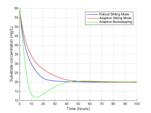
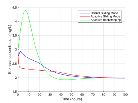
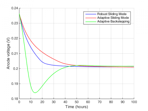
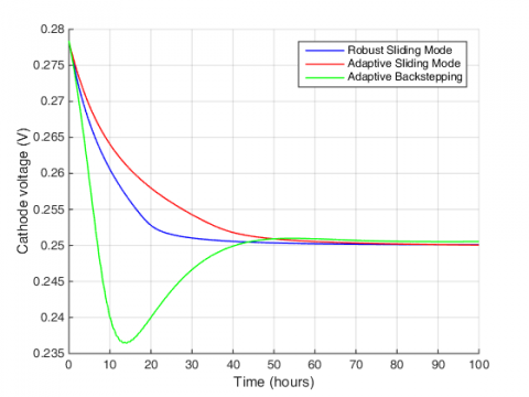
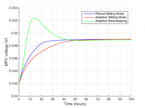
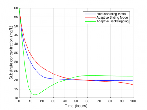
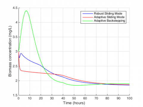
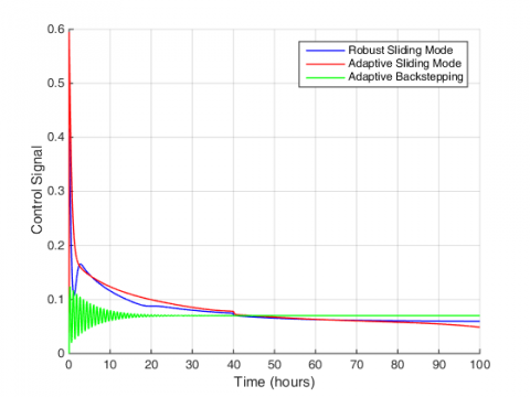
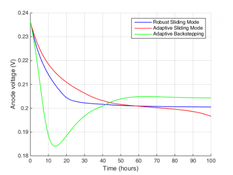
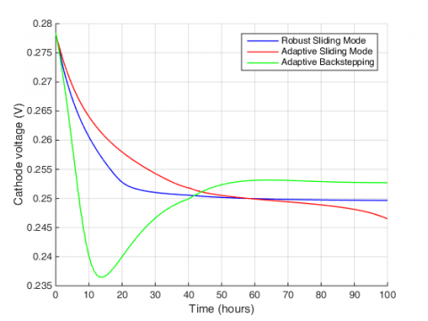
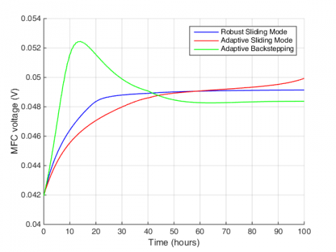
The simulation results are shown in Figures 1 to 6. As can be seen from Figures 1 and 2, using the proposed method, the substrate and biomass concentrations have reached the desired level with higher speed and less error than the adaptive back-stepping and the adaptive sliding mode methods. Also in Figure 3, the control signal obtained from the proposed method shows less amplitude, smoother behavior and of course less fluctuations than the other two methods, and it approaches the final value with a soft behavior and does not experience high speed fluctuations at all. Finally, the output voltages of the anode, cathode, and microbial cell are shown in Figures 4 to 6. From these three Figures, it is clear that the output obtained from the proposed method reaches the final value with smoother behavior, higher speed, less error and without overshoot and undershoot.
Scenario 2. In this scenario, the system has the following parameter uncertainty.
$\left\{\begin{array}{cc}\theta^{-1}=0.4 & \text { if } t<40 \\ \theta^{-1}=0.38 & \text { if } t \geq 40\end{array}\right.$ (28)
The simulation results in this scenario are shown in Figures 7 to 12. The comparison results obtained in the previous scenario are repeated in this scenario. As shown in Figures 7 to 8, the desired substrate and biomass concentrations are well followed. Figure 9 displays that the signal obtained from the proposed control method has less fluctuations than the adaptive back-stepping and adaptive sliding mode methods. Figures 10 to 12 also show the output voltage from the anode, cathode and microbial fuel cell. As in the previous scenario, using the proposed control method, the output voltage without overshoot and undershoot is followed at a higher speed and with smoother behavior compared to adaptive back-stepping and adaptive sliding mode methods. Both of the above scenarios show that the proposed robust sliding mode is well able to track the control targets intended for the microbial fuel cell despite the nonlinear terms and the uncertainty of the system.
Figure 1. Performance of substrate concentration
Figure 2. Performance of biomass concentration
Figure 3. Control Signal
Figure 4. Anode voltages of single chamber MFC
Figure 5. Cathode voltages of single chamber MFC
Figure 6. Voltages of single chamber MFC
Figure 7. Performance of substrate concentration
Figure 8. Performance of biomass concentration
Figure 9. Control Signal
Figure 10. Anode voltages of single chamber MFC
Figure 11. Cathode voltages of single chamber MFC
Table 1. The percentage of overshoot and undershoot values of all responses for all controllers in Scenario 1
|
Controller |
State |
Overshoot |
Undershoot |
|
Adaptive Sliding Mode |
Substrate concentration (mg/L) |
- |
- |
|
Biomass concentration (mg/L) |
- |
- |
|
|
Anode voltages (V) |
- |
- |
|
|
Cathode voltages (V) |
- |
- |
|
|
MFC voltages (V) |
- |
- |
|
|
Adaptive Backstepping |
Substrate concentration (mg/L) |
0.63 |
8.25 |
|
Biomass concentration (mg/L) |
2.40 |
0.08 |
|
|
Anode voltages (V) |
- |
0.02 |
|
|
Cathode voltages (V) |
- |
0.02 |
|
|
MFC voltages (V) |
0.01 |
- |
|
|
Robust Sliding Mode |
Substrate concentration (mg/L) |
- |
- |
|
Biomass concentration (mg/L) |
0.93 |
- |
|
|
Anode voltages (V) |
- |
- |
|
|
Cathode voltages (V) |
- |
- |
|
|
MFC voltages (V) |
- |
- |
Table 2. the percentage of overshoot and undershoot values of all responses for all controllers in Scenario 2
|
Controller |
State |
Overshoot |
Undershoot |
|
Adaptive Sliding Mode |
Substrate concentration (mg/L) |
unstable |
|
|
Biomass concentration (mg/L) |
|||
|
Anode voltages (V) |
|||
|
Cathode voltages (V) |
|||
|
MFC voltages (V) |
|||
|
Adaptive Backstepping |
Substrate concentration (mg/L) |
2.45 |
8.27 |
|
Biomass concentration (mg/L) |
2.40 |
0.02 |
|
|
Anode voltages (V) |
0.004 |
0.02 |
|
|
Cathode voltages (V) |
0.003 |
0.02 |
|
|
MFC voltages (V) |
0.01 |
0.002 |
|
|
Robust Sliding Mode |
Substrate concentration (mg/L) |
- |
- |
|
Biomass concentration (mg/L) |
0.93 |
0.02 |
|
|
Anode voltages (V) |
- |
- |
|
|
Cathode voltages (V) |
- |
- |
|
|
MFC voltages (V) |
- |
- |
|
Figure 12. Voltages of single chamber MFC
To show the superiority of the proposed control method in terms of transient state behavior of the system, its overshoot and undershoot is compared in Tables 1 and 2. As can be seen from the tables, under the proposed controller, the system states experience smoother behavior without overshoot and undershoot. It should be noted that the appropriate transient behavior obtained from the adaptive sliding mode method in Scenario 1 is lost due to instability in Scenario 2.
In this paper, a new robust sliding mode control method is presented for microbial fuel cell system. The control structure is designed to achieve control targets for the microbial fuel cell, while the robust method covers uncertainty and nonlinear term effects. The simulation results in this paper showed the ability of the controller to achieve the desired control objectives, including tracking the desired substrate concentration and of course the constant output voltage. Finite time sliding mode control, simultaneous control of several microbial fuel cells and experimental results can be the path of future studies in this field.
[1] Ardakani, M.N., Gholikandi, G.B., Biomass and Bioenergy, 141, 105726 (2020). https://doi.org/10.1016/j.biombioe.2020.105726
[2] Kim, B.H., Chang, I.S., Gadd, G.M., Applied Microbiology and Biotechnology, 76(3), 485 (2007). https://doi.org/10.1007/s00253-007-1027-4
[3] Slate, A.J., Whitehead, K.A., Brownson, D.A., Banks, C.E., Renewable and Sustainable Energy Reviews, 101, 60 (2019). https://doi.org/10.1016/j.rser.2018.09.044
[4] Menezes, E.J.N., Araújo, A.M., da Silva, N.S.B., Journal of Cleaner Production, 174, 945 (2018). https://doi.org/10.1016/j.jclepro.2017.10.297
[5] Mustapa, M.A., Yaakob, O.B., Ahmed, Y.M., Rheem, C.K., Koh, K.K., Adnan, F.A., Renewable and Sustainable Energy Reviews, 77, 43 (2017). https://doi.org/10.1016/j.rser.2017.03.110
[6] Wang, K., Yuan, B., Ji, G., Wu, X., Journal of Petroleum Science and Engineering, 168, 465 (2018). https://doi.org/10.1016/j.petrol.2018.05.012
[7] Bentsen, N.S., Møller, I.M., Renewable and Sustainable Energy Reviews, 71, 954 (2017). https://doi.org/10.1016/j.rser.2016.12.124
[8] Khare, V., Nema, S., Baredar, P., Renewable and Sustainable Energy Reviews, 58, 23 (2016). https://doi.org/10.1016/j.rser.2015.12.223
[9] Zhong, D., Liao, X., Liu, Y., Zhong, N., Xu, Y., Bioresource Technology, 258, 125 (2018). https://doi.org/10.1016/j.biortech.2018.01.117
[10] Birjandi, N., Younesi, H., Ghoreyshi, A.A., Rahimnejad, M., Journal of Environmental Management, 180, 390 (2016). https://doi.org/10.1016/j.jenvman.2016.05.073
[11] Zeng, Y., Choo, Y.F., Kim, B.H., Wu, P., Journal of Power Sources, 195(1), 79 (2010). https://doi.org/10.1016/j.jpowsour.2009.06.101
[12] Abul, A., Zhang, J., Steidl, R., Reguera, G., Tan, X. Microbial fuel cells: Control-oriented modeling and experimental validation. In 2016 American Control Conference (ACC), 412 (2016).
https://doi.org/10.1109/ACC.2016.7524949
[13] Pinto, R.P., Srinivasan, B., Manuel, M.F., Tartakovsky, B., Bioresource Technology, 101(14), 5256 (2010). https://doi.org/10.1016/j.biortech.2010.01.122
[14] Patel, R., Deb, D., Journal of Power Sources, 396, 599 (2018). https://doi.org/10.1016/j.jpowsour.2018.06.064
[15] Xie, M., Shakoor, A., Li, C., Sun, D., International Journal of Robust and Nonlinear Control, 29(14), 4859 (2019). https://doi.org/10.1002/rnc.4664
[16] Xie, M., Yu, S., Lin, H., Ma, J., Wu, H., IEEE Transactions on Circuits and Systems I: Regular Papers, 67(9), 3199 (2020). https://doi.org/10.1109/TCSI.2020.2981629
[17] Marrani, H.I., Fazeli, S., Malekizade, H., Hosseinzadeh, H., Cogent Engineering, 6(1), 1629055 (2019). https://doi.org/10.1080/23311916.2019.1629055
[18] Fazeli, S., Abdollahi, N., Imani Marrani, H., Malekizade, H., Hosseinzadeh, H., Cogent Engineering, 6(1), 1680093 (2019). https://doi.org/10.1080/23311916.2019.1680093
[19] Ghanavati, M., Salahshoor, K., Motlagh, M.R.J., Ramazani, A., Moarefianpour, A., Journal of Mechanical Science and Technology, 32(2), 823 (2018). https://doi.org/10.1007/s12206-018-0133-1
[20] Alam, W., Ahmad, S., Mehmood, A., Iqbal, J., Indecs, 17(1-B), 85 (2019). https://doi.org/10.7906/indecs.17.1.11
[21] Guo, X., Pan, K., Wang, Q., Wen, Y., IEEE Access, 8, 128096 (2020). https://doi.org/10.1109/ACCESS.2020.3008152
[22] Patel, R., Deb, D., Journal of Power Sources, 434, 226739 (2019). https://doi.org/10.1016/j.jpowsour.2019.226739
[23] Patel, R., Deb, D., Dey, R., Balas, V.E., Adaptive and intelligent control of microbial fuel cells. Springer International Publishing.
[24] Abu-Reesh, I.M., Processes, 8(7), 839 (2020). https://doi.org/10.3390/pr8070839
[25] Fu, X., Fu, L., Marrani, H. I., Journal of Electrical Engineering & Technology, 15(6), 2769 (2020). https://doi.org/10.1007/s42835-020-00535-1
[26] Ortiz-Martínez, V.M., Salar-García, M.J., De Los Ríos, A.P., Hernández-Fernández, F.J., Egea, J.A., Lozano, L.J., Chemical Engineering Journal, 271, 50 (2015). https://doi.org/10.1016/j.cej.2015.02.076
[27] Sheng, H., Huang, W., Zhang, T., Huang, X., Arabian Journal for Science and Engineering, 39(12), 9301 (2014). https://doi.org/10.1007/s13369-014-1448-1