Fatima M. Jasim* | Malik M. A. Al-Isawi | Ali H. Hamad
© 2022 IIETA. This article is published by IIETA and is licensed under the CC BY 4.0 license (http://creativecommons.org/licenses/by/4.0/).
OPEN ACCESS
The spraying operation is one of the most important processes in which industrial robots should be used, the most important of which is spraying for the purpose of painting walls, cars, and devices, in addition to spraying insecticides on plants to get rid of agricultural pests and others. An autonomous spraying robot is intended to alleviate numerous challenges associated with hand spraying. The proposed robot is a wall painting cartesian robot's conceptual design, which includes a paint object with a spray gun and a vision system. The cartesian robot has three links which are X, Y, and Z axes. The spray gun is connected to a screw, which causes the link to move linearly. When the spray gun reaches a particular limit, the camera detects it. The robot needs an appropriate trajectory to prevent collisions with other objects, pass a defined point in spatial coordinates, and accomplish rapid and precise mobility. Through the camera, the robot coordinates mapping, identifies non-sprayable places such as windows or doors and then inspects the spraying effect. The experimental results were applied to four maps (flat map, door map, window map, door and window map, and door and window map), and the corner locations for each map were identified using the vision system. Finally, by comparing the results to the actual distance, the lengths between the corners were computed.
painting wall robot, mathematical models, vision system, path planning and trajectory
Robots are considered one of the most important smart machines that help in many operations because of their quick and accurate achievement compared to human work. In recent years, computer vision systems have developed due to the development of the camera and related algorithms, together with increased demand. These systems use images and videos to understand real-world scenes [1, 2]. In robotics, computer vision techniques can be used, where the camera acts as a sensor for the robot [3]. The camera collects data from the external environment and applies algorithms to the collected data of a particular object to control the applied system [4]. For example, robotic interior wall painting systems are industrial systems that benefit human health and reduce material waste. Computer vision systems can be combined with robots as they influence the robots' trajectory and act as a guide to regulate their movement. First, the data is taken for the external scene. After processing the images, it is possible to deduce the best path that can be applied to the robot according to the specified areas through the images or videos captured through the camera. Images are measured in pixels, and to adjust the robot's path; the units are converted to meters. This is obtained by several algorithms, each of which has advantages and applications, such as Homography, Triangulation, etc. The first step in machine vision is a feature detection that is how find an interest points from the frame, where there are types of interest points such as corner.
In this work, we construct an autonomous spray cartesian robot by examining the above issues and integrating relevant robot structures and modern robot perception technologies. It is developed with a system structure, an environment perception and location module, and a visual detection module. The cartesian robot's contributions can be described as follows: (1) The new mechanical structure design considers the movable robot. (2) By systematically investigating the robot's working environment, the vision system may be tuned to assure accuracy while also achieving real-time operation on the embedded device. A mathematical moder was presented in section 3. In section 4 explains the computer vision system and its connection with robots; section 5 describes the method of planning the robot's movement path; section 6 illustrates the steps of the practical part and simulation results; and section 7 shows the conclusion and future work.
There are studies have been conducted about an automatic spray-painting robot to reach more appropriate results in terms of the type of sensor, the algorithm and the controller used, the motors and the dyeing tool [5, 6]. Scalera et al. [7] developed a painting robot system for graphic and artistic applications based on the anthropomorphic robot with airbrush color pray mathematical model has been introduced based on Gaussian distribution or color intensity. Zaidi et al. [8] proposed a small-scale industry painting robot that can be used in a small factory with the cost being effective. Object recognition has been established in this work-based image processing. The designed robot has a four DOF arm capable of painting different sides of the object. Zhao et al. [9] Proposed a painting robot with a single camera. The estimation scheme for the robot painting parameter process has been implemented. Also, camera calibration has been applied to find its parameters with the wall plane equation. Jiang et al. [10] proposed a cartesian robot with a teach gun based on binocular stereo vision. The data optimization method has been used to remove abnormal values and measurement noise by combing pauta and moving average algorithms. Gao et al. [11] presented spray painting with an intelligent location method using multicamera work on a workpiece positioning system. A modified iterative closest point (ICP) algorithm has been proposed. A 6 DOF pose has been estimated for the painted car part with an estimation of the deformation workpiece. Wang et al. [12] proposed an intelligent spraying robot based on object recognition and a closed-loop control system. The proposed system solves the problem of poor quality and long planning processes caused by the coupler structure workpiece. Tadić et al. [13] proposed a spray painting robot which uses a stereo depth sensor to detect and extract essential information at the surface of objects. Wall information extracting was implemented using morphological operation and image processing algorithms. He et al. [14] designed a spray robot based on inverse P-M diffusion segmentation composed of mechanical, control, and image processing system. Target segmentation has been done using the threshold segment method, where the center coordinates have been extracted.
In this paper, we produced a Cartesian spraying robot using single camera like [9], with using Triangulation method to calculate the distances between corners that is found from vision system algorithm [15].
The robot manipulator is made up of a series of links that are joined together by revolute or prismatic joints; hence it has n+1 links since each joint joins two links. There is a joint variable, indicated by qi, with the joint. qi is the angle of rotation in the case of a revolute joint, and qi is the joint displacement in the case of a prismatic joint [16]. However, the forward kinematics model is an analysis that provides the connection between the individual joints of the robot and the location and orientation of the end-effector. Denavit-Hartenberg's (DH) technique determines the forward kinematics parameters for each link using four variables such as a, d, α, and θ. a represents the link length, d represents the link offset, θ is the joint angle, and α is the joint twist [17]. Cartesian manipulator is one with prismatic first three joints. It contains Cartesian coordinates that reflect the joint variables-the robot's structure and workspace, as illustrated in references [18]. Table 1 presents the D-H parameters of proposed robot, and the matrices of each link are shows below:
Table 1. D-H parameter of robot [18]
|
a |
d |
α |
θ |
|
0 |
q1 |
-90 |
-90 |
|
0 |
q2 |
90 |
-90 |
|
0 |
q3 |
0 |
0 |
$T_1^0=\left[\begin{array}{cccc}1 & 0 & 0 & 0 \\ 0 & 1 & 0 & 0 \\ 0 & 0 & 1 & q_1 \\ 0 & 0 & 0 & 1\end{array}\right], T_2^1=\left[\begin{array}{cccc}1 & 0 & 0 & 0 \\ 0 & 1 & 0 & 0 \\ 0 & 0 & 1 & q_2 \\ 0 & 0 & 0 & 1\end{array}\right],$$T_3^2=\left[\begin{array}{cccc}1 & 0 & 0 & 0 \\ 0 & 1 & 0 & 0 \\ 0 & 0 & 1 & q_3 \\ 0 & 0 & 0 & 1\end{array}\right]$
where, $\mathrm{T}$ is the transformation matrix for the axes of the last frame $O_1 x_1 y_1 z_1$ with respect to the coordinate frame $O_0 x_0 y_0 z_0$ (previous frame) [18]. By multiplying the preceding matrices, the transformation matrix of the endeffector to the reference frame is completed [16, 19]
$T_i^0=T_1^0 \times T_2^1 \times T_3^2$ (1)
$T_3^0=\left[\begin{array}{cccc}1 & 0 & 0 & q_3 \\ 0 & 1 & 0 & q_2 \\ 0 & 0 & 1 & q_1 \\ 0 & 0 & 0 & 1\end{array}\right]$
The joint velocity and joint acceleration of end-effector are calculated with regard to the base frame [20], so:
$V_3^0=\dot{q}_{3 i}-\dot{q}_{2 j}+\dot{q}_{1 k}$ (2)
$a_3^0=\left(\ddot{q}_3-\mathrm{g}\right) i-\ddot{q}_{2 j}+\ddot{q}_{1 k}$ (3)
The equation of motion is derived from the dynamic model. In addition, obtain the system's reaction by employing the state-space model derived from the dynamic equations of robot [21]. Dynamic equations in robot manipulators may be found using a variety of methodologies, including Newton-Euler equations [20].
$m_1 \ddot{q}_{y_1}=F_1-b_1 \dot{q}_{y_1}$ (4)
$m_2 \ddot{q}_{x_1}=F_2-b_2 \dot{q}_{x_1}-k_2 q_{x_1}$ (5)
$m_3 \ddot{q}_{z_1}=F_3-b_3 \dot{q}_{z_1}$ (6)
where, $m_1, q_{y_1}, \dot{q}_{y_1}, \ddot{q}_{y_1}, b_1$, and $F_1$ are the mass, joint position, joint velocity, joint acceleration, damper coefficient, and force applied. The first, second, and third links are denoted by the subscripts $\mathrm{y}_1, x_1$, and $z_1$. The masses are weighted using an appropriate scale to construct the dynamic model of the robot manipulator. The proposed robot consists of three masses. One of them moves vertically and two masses move horizontally [16].
$\left[\begin{array}{ccc}\left(m_1+m_2+m_3\right) & 0 & 0 \\ 0 & \left(m_2+m_3\right) & 0 \\ 0 & 0 & m_3\end{array}\right]\left\{\begin{array}{c}\ddot{q}_{y_1} \\ \ddot{q}_{x_1} \\ \ddot{q}_{z_1}+g\end{array}\right\}+$$\left[\begin{array}{ccc}b_1 & 0 & 0 \\ 0 & b_2 & 0 \\ 0 & 0 & b_3\end{array}\right]\left\{\begin{array}{l}\dot{q}_{y_1} \\ \dot{q}_{x_1} \\ \dot{q}_{z_1}\end{array}\right\}+\left[\begin{array}{ccc}0 & 0 & 0 \\ 0 & K_2 & 0 \\ 0 & 0 & 0\end{array}\right]\left\{\begin{array}{l}q_{y_1} \\ q_{x_1} \\ q_{z_1}\end{array}\right\}=\left[\begin{array}{l}F_1 \\ F_2 \\ F_3\end{array}\right]$ (7)
The equations of motion for each link are shown above; however, to simulate those equations, use the state-space model as follows [22]:
$q_{y_2}=\dot{q}_{y_1}$ (8)
$q_{x_2}=\dot{q}_{x_1}$ (9)
$q_{z_2}=\dot{q}_{z_1}$ (10)
The state matrix given by:
$\left[\begin{array}{c}\dot{q}_{y_1} \\ \dot{q}_{y_2} \\ \dot{q}_{x_1} \\ \dot{q}_{x_2} \\ \dot{q}_{z_1} \\ \dot{q}_{z_2}\end{array}\right]=\left[\begin{array}{cccccc}0 & 1 & 0 & 0 & 0 & 0 \\ 0 & \left(\frac{-b_1}{m_1+m_2+m_3}\right) & 0 & 0 & 0 & 0 \\ 0 & 0 & 0 & 1 & 0 & 0 \\ 0 & 0 & \left(\frac{-K_2}{m_2+m_3}\right) & \left(\frac{-b_2}{m_2+m_3}\right) & 0 & 0 \\ 0 & 0 & 0 & 0 & 0 & 1 \\ 0 & 0 & 0 & 0 & 0 & \left(\frac{-b 3}{m_3}\right)\end{array}\right]$$\left\{\begin{array}{l}q_{y_1} \\ q_{y_2} \\ q_{x_1} \\ q_{x_2} \\ q_{z_1} \\ q_{z_2}\end{array}\right\}$
$+\left[\begin{array}{cccccc}0 & 0 & 0 & 0 & 0 & 0 \\ 0 & \left(\frac{1}{m_1+m_2+m_3}\right) & 0 & 0 & 0 & 0 \\ 0 & 0 & 0 & 0 & 0 & 0 \\ 0 & 0 & 0 & \left(\frac{1}{m_2+m_3}\right) & 0 & 0 \\ 0 & 0 & 0 & 0 & 0 & 0 \\ 0 & 0 & 0 & 0 & 0 & \left(\frac{1}{m_3}\right)\end{array}\right]\left\{\begin{array}{c}0 \\ F_1 \\ 0 \\ F_2 \\ 0 \\ \left(F_3-m_3 g\right)\end{array}\right\}$
Depending on the technique used, robot vision technology allows robots to find, identify, and estimate distance. This research shows a 3DOF cartesian robot that can paint walls. To complete this task, it is necessary to identify whether the wall is a flat surface, its measurements, and the placement of any doors or windows. Then, it assists the robot in moving in the appropriate direction. As a result, the edges and corners of the door, window, and wall must be discovered and detected. If the wall, window, and door are square or rectangular, it will be easier to detect corners than edges because edges have a lot of points. Still, corners have a few points that can collect them, reducing the amount of observed data and simplifying classification. Various approaches, including Harris, SIFT, and SURF, can be used to locate and retrieve an item. After that, the required corners are determined, and the points value is extracted in pixel units [23].
4.1 Harris corner detector
It is a method for identifying corner points where moving the window in any direction should result in a considerable change in intensity of pixel. Finding the location of objects using interest points is required and effective since these points remain in the exact location when changed with a minor variation in values that can be quantified and predicted. As a result, corner points are an important form of interest point. However, estimating position in a flat environment is difficult due to the lack of interest points. As shown in Figure 1, if region is a flat, there is no change in all directions, while if it is an edge, there is no change along the edge direction, and in the corner, there is a significant change in all directions with a small shift. Harris corner detector is invariant in transformed location and shifting image and covariant in scaling.
Figure 1. Different types of image regions
Figure 2. Steps of Harris Corner Detector
The steps to find the Harris corner detector of an image numerically are described in chart as shown in Figure 2.
$E(u, v)=\sum_{x, y} w(x, y)[I(x+u, y+v)-I(x, y)]^2$ (12)
where, $I(x, y)$ is the original image, $I(x+u, y+v)$ is the shifted intensity image, $u$ and $v$ are the value of shifting in $x$ and y. By applying Taylor Expansion series and some mathematical steps to equation (12) it become as follows [24, 25]:
$E(u, v)=[u v]\left(\sum\left[\begin{array}{cc}I_x^2 & I_x I_y \\ I_x I_y & I_y^2\end{array}\right]\right)\left[\begin{array}{l}u \\ v\end{array}\right]$ (13)
$I_x$ and $I_y$ are found from derivative the image with $\mathrm{x}$ and $\mathrm{y}$, the second matrix named M matrix. Then solving SSD of equation by find eigenvector of $\mathrm{M}$ matrix as follows:
$M-\lambda I=0$ (14)
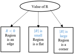
$R=\operatorname{Det}(M)-K(\operatorname{trace}(M))$ (15)
where, $\operatorname{det}(\mathrm{M})=\lambda_1 \lambda_2$, trace $=\lambda_1+\lambda_2$, and $\mathrm{k}$ is between $0.04-$ $0.06, \lambda 1$ and $\lambda 2$ are the eigenvalues of $\mathrm{M}$ matrix and values of them give the decision of type of region, as shown in Figure 3.
Figure 3. Classification of regions
4.2 Position estimation
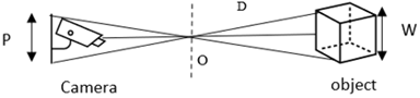
Position estimation is an important robotics approach involving a computer vision system. The significance is that it aids in estimating the robot's movement based on the estimated positions. The positions that must be estimated to facilitate the robot's mobility are the barriers to avoid and the destinations to reach. Several significant approaches are employed to estimate positions, including Homograph, Fundamental, and Triangulation. The modified triangulation method is one of the most recent and fastest in the field of position estimation; as illustrated in Figure 4, it requires knowing the focal length of the camera (f), the distance between the camera and the object (D), and the value of the distance that the camera reads in pixels (p). There is a distance between the camera and the item, the value determined by the object's size. To calculate the percentage error, apply more than one distance value and compare them. The modified triangulation approach is used to solve the following problems [15]:
$W=D \times \frac{P}{F}$ (16)
where, W denotes the needed real area of an item, D denotes the distance between the camera and the object, P is the area measured in pixel units by the camera, and F denotes the focal length of the camera, which may be in the x or y direction depending on the required area.
Figure 4. Relationship between camera and object
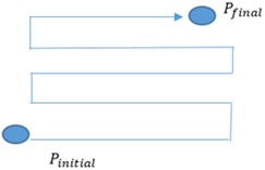
Path planning is an algorithm that presents a set of points (a set of joint variables) that connects a start and a goal. Therefore, it just describes the robot's location without any dynamic motion features, as illustrated in Figure 5. On the other hand, the trajectory is a planned motion that includes time information (position, velocity, and acceleration). Many algorithms are available, including cubic polynomial, quantic polynomial, linear segment parabolic mix, and minimal time trajectory [16]. In addition, numerous approaches describe the robot's trajectory, including joint and Cartesian space. In robotics, the joint-space trajectory is a standard method for achieving smooth, continuous travel between two sets of joint angles. Cartesian space, on the other hand, is a way for the trapezoid velocity curve with parabolas meant to make the acceleration continuous.
Figure 5. path planning of robots
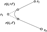
The path begins at $\left(r_o\right)$ at time $\left(t_o\right)$ and proceeds along a line with constant speed $\left(v_1\right)$ until it researches a location at switching time $\left(t_1-t^{\prime}\right)$. At this point, the path transforms into a continuous acceleration parabola. Then, the path shifts to the second line at time $\left(t_1+\mathrm{t}^{\prime}\right)$ and proceeds with uniform speed $\left(v_2\right)$ towards to the goal at point $\left(r_2\right)$. If there were no transition path, the time $\left(t_1-t_o\right)$ is necessary to move from $\left(r_o\right)$ to $\left(r_1\right)$, and the time $\left(t_2-t_1\right)$ is required to move from $\left(r_1\right)$ to $\left(r_2\right)$. Figure 4 depicts the path schematically. To execute Figure 6 using the parabola approach, the interval must be segmented into three parts of position trajectory, such as the first line from $\left[r_o-r\left(t_1-t^{\prime}\right)\right]$, the parabola curve from $\left[r\left(t_1-t^{\prime}\right)\right.$ $\left.r\left(t_1+t^{\prime}\right)\right]$, and the second line from $\left[r\left(t_1+t^{\prime}\right)-r_2\right]$. Because the first and second lines are not deformed, they are provided by Eq. 17. Eqns. (17)-(23) are depicted by [26]:
$r(t)=\left\{\begin{array}{ll}r_1-\frac{t_1-t}{t_1-t_0}\left(r_1-r_0\right) & {\left[t_0 \leq t \leq t_1\right]} \\ r_2-\frac{t_1-t}{t_2-t_1}\left(r_2-r_1\right) & {\left[t_1 \leq t \leq t_2\right]}\end{array}\right\}$ (17)
where, $r_o, r_1$, and $r_2$ are a q-points of the robot path, $t_o$ is initial time, $t_1$ is the time taken to reach point $r_1$, and $t_2$ is the final time when the goal is reached. But for parabola curve, a switching time is important to implement parabolas to avoid squeaky corners. Wherefore there are two times $\left(\left(t_1-t^{\prime}\right)\right.$ and $\left.\left(t_1+t^{\prime}\right)\right)$ to replace between line and curve and vice versa. So, the curve equation is given by:
$r(t)=r_1-\delta_1 \frac{\left(t-t^{\prime}-t_1\right)^2}{4 t^{\prime}\left(t_1-t_o\right)}+\delta_2 \frac{\left(t+t^{\prime}-t_1\right)^2}{4 t^{\prime}\left(t_2-t_1\right)}$ (18)
where, $\delta_1$ is equal to $r_1-r_0$, and $\delta_2$ is equal to $r_2-r_1$.
While the velocity of trajectory planning is segmented into three areas the first and second lines have become a constant line [26], and the parabola curve is given by:
$\dot{r}\left(t_1-t^{\prime}\right)=\frac{1}{t_1-t_o} \delta_1$ (19)
$\dot{r}\left(t_1-t^{\prime}\right)=\frac{1}{\left(t_2-t_1\right)} \delta_2$ (20)
Beside that for acceleration motion, assume it is constant along transition curve [26] and after integrated is given by:
$\ddot{r}_c=\frac{1}{2 t^{\prime}}\left(\frac{\delta_2}{\left(t_2-t_1\right)}-\frac{\delta_1}{\left(t_1-t_o\right)}\right)$ (21)
Figure 6. Transition between two lines segments as a path in Cartesian space
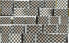
As described in previous sections, the suggested robot is of the cartesian type and moves in three directions (X, Y, Z), so the camera was put on the second joint of the robot between the second and third links, as illustrated in Figure 7. More information on this robot can be found in reference [18]. In this work, a camera calibration process begins with capturing a series of images for the chessboard as shown in Figure 8 and then employing an algorithm to extract K-matrix that includes the focal length and principal points.
A computer vision system is required. In this project, we began with camera calibration using a USB webcam model Microsoft LifeCam HD-3000, as shown in Table 2. This procedure was carried out using chessboard paper. Camera calibration is a critical step in determining intrinsic and extrinsic camera properties.
Figure 7. Cartesian robot with USB web Camera
Table 2. Microsoft LifeCam HD-3000 specifications
|
Specification |
Value |
|
Product Name |
HD-3000 Microsoft LifeCam |
|
Length |
39.3 mm |
|
Width |
44.5 mm |
|
Depth/Height |
109 mm |
|
Weight |
89.9 g |
|
Interface |
High-speed USB compatible with USB 2.0 |
|
Rate of Image |
More than 30 frames/sec. |
|
Field of View |
68.5° diagonal field of view |
|
Fixed focus |
(0.3m- 1.5m) |
|
True Color |
Automatic image adjustment with manual override |
|
Features of Image |
16:9 widescreen 24-bit color depth |
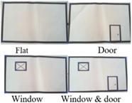
When finding the image parameters, the focal length and intrinsic matrix are sorted to be used later. Following that, four maps are suggested, including the flat, door, window, and window with door maps, as shown in Figure 9. It applies the Harris corner detector to extract the specific points. After separating the essential points from others, the required areas are estimated in the world coordinate system. Finally, the distance estimated between an object to other is calculated by using the triangulation method. Finally, trajectory planning was conducted after segmented path planning based on the sort of map and the barriers it contained.
Figure 8. Calibration of chessboard pictures
Figure 9. chosen maps
6.1 Camera calibration
The camera calibration process begins with capturing a series of images for the chessboard depicted in Figure 7, followed by the use of an algorithm to extract a K matrix (Intrinsic Matrix) that includes the focal length and principal points, external parameters, and reprojection errors for each image, as depicted in Figures 10 and 11.
$K=\left[\begin{array}{ccc}1233.7 & 0 & 650.3 \\ 0 & 1236.9 & 371.4 \\ 0 & 0 & 1\end{array}\right]$
The focal length of the X-direction as 1233.7, the focal length of the Y-direction as 1236.9, and the primary points (U, V) as (650.3, 371.4) are presented in K matrix.
Figure 10. Reprojection errors of calibration pictures
Figure 11. Extrinsic parameters of camera calibration
6.2 Vision validation
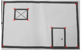
In this work, four map scenarios were taken for three different distances between the camera and the map (40 cm, 45 cm, and 50 cm) to calculate the corners of the pictures using the Harris detector. First, the interest points of the proposed maps were extracted, as shown in Figure 12, for the door and window maps. Then, after defining the interest points of the corners for each map, the distances between them for each map were determined by first calculating the distances realistically and fixing their values.
Figure 12. Corners Detector features
Scenario 1: As illustrated in Figure 13 for the flat map, two distances, a and b, must be determined in the world dimensions based on the predicted position. Then, the results are compared to the distance for three chosen depths, as shown in Table 3.
Figure 13. Flat map
Table 3. Flat map results
|
Depth |
Distance |
Estimated data |
Real data |
Percentage Error |
|
D=40 cm |
a |
34.631 |
37.5 |
7.6494 |
|
b |
20.535 |
22.5 |
5.2408 |
|
|
D=45 cm |
a |
34.002 |
37.5 |
9.3279 |
|
b |
19.771 |
22.5 |
7.2764 |
|
|
D=50 cm |
a |
36.667 |
37.5 |
2.2208 |
|
b |
22.326 |
22.5 |
0.46475 |
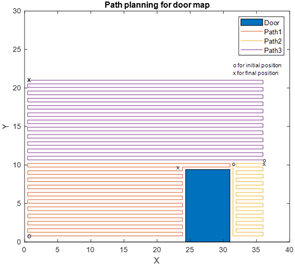
Scenario 2: Only the door is an obstacle on this map. As illustrated in Figure 14 and Table 4, four distances, a, b, c, and d, were computed and compared to the actual distance.
Figure 14. Door map
Table 4. Door map results
|
Depth |
Distance |
Estimated data |
Real data |
Percentage Error |
|
D=40 cm |
a |
23.227 |
24.5 |
5.198 |
|
b c d |
6.6907 5.017 8.9861 |
7 6 9.5 |
1.2624 4.0122 2.0975 |
|
|
D=45 cm |
a |
22.553 |
24.5 |
7.9483 |
|
b c d |
6.7702 5.4509 9.0673 |
7 6 9.5 |
0.93785 2.2411 1.7661 |
|
|
D=50 cm |
a |
24.297 |
24.5 |
0.83005 |
|
b c d |
6.6868 5.4593 9.4236 |
7 6 9.5 |
1.2784 2.2071 0.31165 |
Scenario 3: The third map-only window in our computation, as shown in Figure 15, and the outcome is displayed in Table 5.
Figure 15. Window map
Table 5. Window map results
|
Depth |
Distance |
Estimated data |
Real data |
Percentage Error |
|
D=40 cm |
a |
4.5391 |
5.4 |
3.4574 |
|
b c d e f |
6.1456 20.871 11.536 5.0559 2.5338 |
7.2 24.9 13.3 6 3.2 |
4.2344 16.18 7.0853 3.7916 2.6753 |
|
|
D=45 cm |
a |
4.9344 |
5.4 |
1.87 |
|
b c d e f |
6.3688 23.699 12.842 5.2603 2.6228 |
7.2 24.9 13.3 6 3.2 |
3.3383 4.8223 1.8407 2.9706 2.318 |
|
|
D=50 cm |
a |
5.0797 |
5.4 |
1.2862 |
|
b c d e f |
6.7599 22.82 12.71 5.5117 2.8799 |
7.2 24.9 13.3 6 3.2 |
1.7674 8.3527 2.369 1.9609 1.2857 |
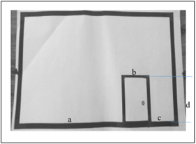
Scenario 4: As seen in Figure 16, the final map includes a window and a door in our estimate. Table 6 shows the experimental results.
According to our calculations and algorithm used in this work, the best depth that can be obtained is 45 cm, and the result for all cameras is satisfactory, with a percentage error of less than 9%.
Figure 16. Window and door
Table 6. Window and Door map results
|
Depth |
Distance |
Estimated data |
Real data |
Percentage Error |
|
D=40 cm |
a |
4.931 |
5.4 |
3.9086 7.3963 10.798 7.4093 5.0996 9.0347 2.9749 6.8713 4.5146 |
|
b c d e f g h i |
6.31241 10.704 6.1109 5.288 8.4158 3.443 5.1754 2.6583 |
7.2 12 7 5.9 9.5 3.8 6 3.2 |
||
|
D=45 cm |
a |
4.988 |
5.4 |
3.4329 |
|
b c d e f g h i |
6.2011 10.613 6.4995 5.4217 8.6001 3.5929 5.0604 2.5332 |
7.2 12 7 5.9 9.5 3.8 6 3.2 |
8.3239 11.559 4.1707 3.9858 7.4995 1.726 7.83 5.557 |
|
|
D=50 cm |
a |
4.7429 |
5.4 |
5.4759 |
|
b c d e f g h i |
6.3389 10.514 6.0432 5.164 8.2929 3.1738 5.0755 2.6133 |
7.2 12 7 5.9 9.5 3.8 6 3.2 |
7.1759 12.38 7.9731 6.1335 10.059 5.2185 7.7045 4.889 |
Figure 17. Path planning of map 1
Figure 18. Path planning of map 2
Figure 19. Path planning of map 3
Figure 20. Path planning of map 4
6.3 Spray painting path planning
Path Planning has been suggested for each map based on the obstacles it presents. Consequently, the maps were split based on the regions computed in the findings, with a 0.5 distance from the points assumed for safe spraying. Because map 1 (flat map) lacks obstacles, a single path was proposed, as illustrated in Figure 17, that begins at a location (0.5,0.826) and ends at a point (0.5,0.826). (36.17,21.83). While the other maps contain obstacles, three paths have been suggested for map 2 (door only), as shown in Figure 18. The first path in orange color starts from a point (0.47,0.799) and ends at a point (23.36,9.73), the second path in violet color starts from (0.47,21.01) and ends at (35.97,10.76), and the last path in yellow color starts from a point (35.97,10.2) and ends in point (35.97,10.76 (31.45,10.2). As for map 2 (Window only), four paths were suggested, as shown in Figure 19. The first path, in orange, begins at (0.5,0.5) and ends at (34.16,12.5). The second path, in yellow, begins at (34.16,12.71) and ends at (12.34,20.7). Then the third path, in purple, begins at (12.04,20.7) and ends at (0.5,18.7). Finally, the fourth path, in green, begins at (0.5, 18.2) and (0.5, 12.7). Figure 20 depicts six paths for the window and door map (map4). The first path (yellow color) begins at (0.5,0.5) and ends at (4.488,19.5), whereas the second way (violet color) begins at (4.988,19.5) and ends at (4.488,19.5). (4.988,18). The third green-color route begins at (11.69,17.25) and ends at (33.22,9.253). Furthermore, the fourth path (cyan color) begins at (33.22,8.6) and finishes at (28.8,0.6001), while the fifth way (red color) begins at (21.3,8.6) and ends at (28.8,0.6001). (11.19,0.6001). The final path (blue color) begins at (10.69,0.5) and concludes at (5.488,11.69).
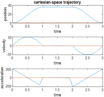
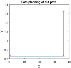
Figure 21. Trajectory of Cartesian path
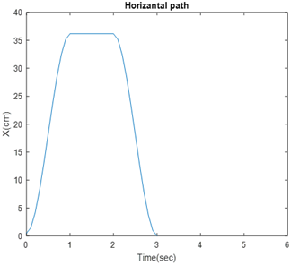
Figure 22. Profile of the path
Figure 23. X-position w.r.t time
Figure 24. Y-position w.r.t time
6.4 Trajectory
The Cartesian path is a repetitive zigzag rectangular form, as depicted in Figures 17-20. As a result, the flat map was chosen and deducted the first four points from it to complete the trajectory planning to obtain the position, velocity, and acceleration through time, as shown in Figure 21. The path of chosen points, a horizontal path with respect to time, and a vertical path concerning time are shown in Figures 22-24, respectively.
The robot structure of spraying cartesian robot is designed to be durable and suitable for the required movement. A visual system guiding the painting cartesian robot was presented in this work. This system employed a precise approach for finding the actual distances and reducing the percentage error. Four wall maps were chosen in this work, with the entrance's rectangular form and the window's square acting as the standard shape. The Harries and triangulation methods were used to identify map corners and compute distances. An acceptable result was gathered utilizing the vision system approach at different depths (40, 45 and 50 cm). The suitable depth is found at 45 with 11.559%. The trajectory for horizontal and vertical movements is presented; position, velocity, and acceleration results are acceptable, and the path planning is smooth. Spray painting robots have contributed to many benefits, including reducing the consumption of the material, the speed and accuracy of work, and the lack of direct exposure of the person, thus affecting health. In future work, more variable maps and shapes of doors and windows can be used, and as a result, boundary and angle detectors are used together to calculate distances in real-time. It is also possible to enhance the robot's work by making it a mobile robot by adding (2DOF) to complete its work accurately without human intervention. Besides that, it can be to complete its work in real time without need to Pre-analysis of maps by programming it by python to work online. Where the camera captures an image for the wall, then the controller receives the data to recognition what kind of map it is and calculate the distances between corners to move the robot according to the given data.
This work is supported by Department of Mechatronics engineering in Al-Khwarizmi college of engineering at university of Baghdad.
[1] Zhou, L., Zhang, L., Konz, N. (2023). Computer vision techniques in manufacturing. IEEE Transactions on Systems, Man, and Cybernetics: Systems, 53(1): 105-117. https://doi.org/10.1109/TSMC.2022.3166397
[2] Banús, N., Boada, I., Xiberta, P., Toldrà, P. (2022). Design and Deployment of a Generic Software for Managing Industrial Vision Systems. IEEE Transactions on Automation Science and Engineering, 19(3): 2171-2186. https://doi.org/10.1109/TASE.2021.3078787
[3] Rivera-Calderón, S., Lázaro, R.P.S., Vazquez-Hurtado, C. (2022). Online assessment of computer vision and robotics skills based on a digital twin. IEEE Global Engineering Education Conference (EDUCON), pp. 1994-2001. https://doi.org/10.1109/EDUCON52537.2022.9766459
[4] Hamad, A.H. (2021). Smart campus monitoring based video surveillance using haar like features and k-nearest neighbour. International Journal of Computing and Digital Systems, 10(1): 79. http://dx.doi.org/10.12785/ijcds/100179
[5] Xu, Y., Zhang, H., Cao, L., Shu, X., Zhang, D. (2022). A shared control strategy for reach and grasp of multiple objects using robot vision and noninvasive brain–computer interface. IEEE Transactions on Automation Science and Engineering, 19(1): 360-372. http://dx.doi.org/10.1109/TASE.2020.3034826
[6] Ravigopal, S.R., Brumfiel, T.A., Sarma, A., Desai, J.P. (2022). Fluoroscopic image-based 3-D environment reconstruction and automated path planning for a robotically steerable guidewire. IEEE Robotics and Automation Letters, 7(4): 11918-11925. http://dx.doi.org/10.1109/LRA.2022.3207568
[7] Scalera, L., Mazzon, E., Gallina, G., Gasparetto, A. (2017). Airbrush robotic painting system: Experimental validation of a colour spray model. Advances in Service and Industrial Robotics, Adria-Danube Region, pp. 549-556. https://doi.org/10.1007/978-3-319-61276-8_57
[8] Zaidi, S.M.K., Junejo, F., Mujtaba, S.B. (2017). Computer aided design of a low-cost painting robot. Mehran University Research Journal of Engineering & Technology, 36(4): 841-856. https://doi.org/10.3316/informit.238140763686517
[9] Zhao, Q., Li, X., Lu, J., Yi, J. (2018). Monocular vision-based parameter estimation for mobile robotic painting. IEEE Transaction Oninstrumentation and Measurement, 68(10): 3589-3599. https://doi.org/10.1109/TIM.2018.2878427
[10] Jiang, C., Li, X., He, W., Kou, C., He, J. (2019). Research on teaching system for painting robot based on binocular stereo vision. IEEE 5th International Conference on Computer and Communications, Chengdu, China, pp. 1754-1758. https://doi.org/10.1109/ICCC47050.2019.9064467
[11] Gao, H., Ye, C., Lin, W., Qiu, J. (2020). Complex workpiece positioning system with nonrigid registration method for 6-dofs automatic spray painting robot. IEEE Transactions on Systems, Man, and Cybernetics: Systems, 51(12): 2168-2216. https://doi.org/10.1109/TSMC.2020.2980424
[12] Wang, Z.F., Zhen, Z.M., Lin, Z.Q., Wen, T., Guo, C.L., Chen, H.C. (2020). An adaptive industrial robot spraying planning and control system. In IECON 2020 The 46th Annual Conference of the IEEE Industrial Electronics Society, Singapore, pp. 1739-4743. https://doi.org/10.1109/IECON43393.2020.9254323
[13] Tadić, V., Odry, A., Burkus, E., Kecskés, I., Király, Z., Vízvári, Z., Tóth, A., Odry, P. (2021). Application of the ZED depth sensor for painting robot vision system development. IEEE Access, 9: 117845-117859. https://doi.org/10.1109/ACCESS.2021.3105720
[14] He, Z., Cui, L., Zhao, S. (2022). A novel inverse p-m diffusion enhanced code spraying robot for express security inspection. IEEE Access, 10: 32350-32360, https://doi.org/10.1109/ACCESS.2022.3160731
[15] Lee, J.M. (2021). Real distance measurement using object detection of artificial intelligence. Turkish Journal of Computer and Mathematics Education (TURCOMAT), 12(6): 557-563. https://doi.org/10.17762/turcomat.v12i6.1979
[16] Spong, M.W., Hutchinson, S., Vidyasagar, M. (2020) Robot Modeling and Control. John Wiley & Sons.
[17] Siciliano, B., Sciavicco, L., Villani, L., Oriolo, G. (2009). Force Control. Springer London.
[18] Fatima, M., Jasim, M., Ali, M., Hamad, A.H. (2022). Design and analysis of a spraying robot. Al-Khwarizmi Engineering Journal, 18(3): 1–14. https://doi.org/10.22153/kej.2022.07.001
[19] Abaas, T.F., Khleif, A.A., Abbood, M.Q. (2020). Inverse kinematics analysis and simulation of a 5 DOF robotic arm using MATLAB. Al-Khwarizmi Engineering Journal, 16(1): 1-10. https://doi.org/10.22153/kej.2020.12.001
[20] Belay, T.T. (2017). Mathematical modeling and dynamic simulation of gantry robot using bond graph. International Conference on Information and Communication Technology for Develoment for Africa, Bahir Dar, Ethiopia, pp. 228-237. https://doi.org/10.1007/978-3-319-95153-9_22
[21] Ljung, L., Glad, T. (2002). Modeling of Dynamic Systems. Prentice-Hall, Inc.
[22] Burns, R. (2001). Advanced Control Engineering. Elsevier.
[23] Al-Isawi, M., Sasiadek, J.Z. (2019). Pose estimation for mobile and flying robots via vision system. Aerospace Robotics III, pp. 83-96. https://doi.org/10.1007/978-3-319-94517-0_6
[24] Sikka, P., Asati, A.R., Shekhar, C. (2021) Real time FPGA implementation of a high speed and area optimized Harris corner detection algorithm. Microprocessors and Microsystems, 80: 103514. https://doi.org/10.1016/j.micpro.2020.103514
[25] Elliott, J., Khandare, S., Butt, A.A. (2022). Automated tissue strain calculations using harris corner detection. Annals of Biomedical Engineering, 50(5): 564-574. https://doi.org/10.1007/s10439-022-02946-9
[26] JAZAR, R.N. (2010). Theory of Applied Robotics: Kinematics, Dynamics, and Control. Springer.