Maha Raad Hassan* | Shibly Ahmed Al-Samarraie
© 2022 IIETA. This article is published by IIETA and is licensed under the CC BY 4.0 license (http://creativecommons.org/licenses/by/4.0/).
OPEN ACCESS
Control of Heating, Ventilating, and Air Conditioning (HVAC) aims to provide a comfortable environment for human life in terms of temperature and humidity and improve indoor air quality. The HVAC system is multi-input multi-output, where the control design of this system is challenging due to its strong nonlinearity and the coupled influence of both system controllers on the temperature within the thermal zone. The aim of this study is to design a dual-controller for the HVAC system. The first controller is a non-linear feedback controller which is devoted to control the humidity ratio of the thermal zone with the desired characteristic. While for the second one, a robust controller is designed to maintain the desired thermal zone temperature based on the adaptive sliding mode controller (ASMC). Using the ASMC enabled us to design the second controller without the need to know the uncertainty bound on the HVAC system model. Additionally, the stability of the proposed control system was verified using the Lyapunov theory. To construct the sliding variable for the temperature control, the error state which is the difference between the thermal zoon temperature and the desired value and its derivative is needed. Due to the uncertainty in the error state derivative, a robust differentiator was designed using the approximate classical sliding mode differentiator (ACSMD). Finally, the performance of the control system is confirmed via numerical simulation. The results showed the robust ability of the control system to make the humidity and temperature of the thermal area follow the required values and with high accuracy.
adaptive sliding mode control, feedback continuous control, HVAC systems, MIMO systems, robust control
HVAC systems are the major energy-consuming devices in buildings. The building section utilizes about 74% of the electricity consumption, and more than 56% of this utilization was supposed to the HVAC systems [1]. Any bettering can result in lowering demand during peak load periods of the day. While many studies have been directed on enhancement the design of equipment and building envelopes.
Data-driven HVAC can identify strategies for system clarification and enhancement which is termed system identification (SI) in the literature [2]. Data was used to create a mathematical-based HVAC system which examine input and output variables to identify and set system parameters [3].
The impact of Neighboring zones on temperature tracking and control effort because of heat transfer was proposed by conduction through separating surfaces where heat transfer impact was reduced through feedback linearization scheme [4].
A precise model of the building is essential for the design of a complicated HVAC system. Heat dynamics of a space can be represented by the zone model, the comfortable zone which is controlled by an air-handling unit (AHU) or an air-terminal device [5].
The temperature and humidity are the most common parameters of HVAC system. Which controlled through airflow and water flow control. The capability of variable air volume (VAV) in HVAC systems are 15–40% more energy efficient than constant volume HVAC systems [6]. The wavlet artificial based neural network with infinite impulse response filter was proposed by Jahedi and Ardehali [7] for the faster and accurate identification of system dynamics to control the temperature and humidity of thermal zone. The result showed that, the used control can improve energy efficiency when compared with the proportional derivative (PD) controller. Two control strategies (gain scheduling and feedback linearization) were applied to a nonlinear dynamic model of an AHU and analyzed the strength and weakness of each approach [8]. A dynamic extension algorithm is employed to HVAC system, which its modeling including CO2 concentration [9]. The linear quadratic regulator (LQR) was applied to optimize an stabilize the system. The unscented Kalman filter relies on scaled unscented transformation (UT) is used in the Ref. [10] to specify a state estimation of AHU which is controlled through a linear quadratic regulator, and without linearization to reduce mistakes to keep scheme features. The state dependent Riccatti Equation with the pseudo linearization was proposed, which is used for designing observer and sub-optimal controller for the AHU and compared with the extended Kalman filter [11]. A fuzzy controller was proposed by Shah et al. [12] with distinct type and number of membership functions and investigated which shape can give desired performance with energy consumption this controller is compared with variety controllers including self-tuning adaptive fuzzy controller, LQR and nonlinear controllers. A neural fuzzy structure of a parameter self-tuning decoupled fuzzy neural PID controller was proposed by Ganchev et al. [13]. A nonlinear model predictive control approach according to an optimization function is used on iterative optimization with a finite horizon and it can generate a control signal regardless of a past error [14]. Robustness of a control system is crucial because of dynamic uncertainties and external disturbances [15].
Sliding-mode control (SMC) is known as appropriate strategy for its robustness against external disturbances and insensitivity to parameter variations under matching conditions during sliding mode [16]. The SMC needs a proper control law such trajectory moves toward the sliding surface and reaches in a finite time and stays on. Sliding mode control is introduced by Shah et al. [17]. The proposed controller performance compared with performance of PID controller to prove the advantage of using SMC to improving the desired tracking was shown in the paper [18]. But the large control gains that used with conventional SMC which cause undesired chattering while the control system is in the sliding mode which is the major disadvantage of SMC [19]. Chattering can usually be attenuated by choosing appropriate control gain according to a certain adaptation law and that reducing also the control effort.
In this work, a nonlinear controller is used for controlling the humidity ratio and a controller based on an adaptive sliding mode controller to control the temperature of the thermal zone. An adaptive sliding mode control methodology is proposed by Plestan et al. [20] which guarantees a real sliding mode. Adaptive sliding mode control is introduced for many applications like for heat exchanger as in the paper [21].
The structure of this article is as follows: Firstly, the problem statement and proposed controller design is introduced in section 2, while the HVAC system description and modeling is presented in section 3. SMC is presented in section 4. Then the controllers design is explained in section 5. The simulation results are discussed in section 6. Finally, section 7 contains the conclusion.
The HVAC system is a multi-input multi-output system (MIMO), where the control inputs in our case study, are the flow rate of the air, and the flow rate of the water. While the outputs are the temperature and the humidity of the thermal zone.
HVAC system’s features are MIMO, non-affine, difficult nonlinearities, time-varying, complicated models and coupling between control variables [22]. designing advanced control techniques concerning the characteristics of the system is required. Consequently, so linear control cannot be an appropriate choice to obtain a desirable performance and stability level solutions with nonlinear behavior and time-varying characteristics of the system
The control system design proposed in this paper suggested splitting the dynamic model into two parts, the upper part which is responsible for the stabilization of humidity is controlled using nonlinear feedback continuous controller. While for the lower part, which is responsible for stabilizing the indoor temperature, the adaptive sliding mode controller with approximate signum function is proposed. In order to compute the sliding variable, the time derivative of an error function that computed the difference between the indoor temperature and the desired temperature is needed. But due to the uncertainty in the HVAC system model, the estimation of derivatives of the error function is estimated here via the ACSMD.
The single thermal zone HVAC system with VAV and Variable Water Flow capabilities in cooling mode is showed in Figure 1. It consists of the following components: a heat exchanger; a chiller, which provides chilled water to the heat exchanger; a circulating air fan; the thermal space; connecting ductwork; dampers; and mixing air components [23].
Figure 1. HVAC drawing view with single thermal zone in the VAV system
The operation process of air conditioning system on cooling mode is consist of five stages as clarified in Figure 1:
Fresh air is allowed to enter the system by $\ell \%, \ell<1$ and mixed with circulated air, which is $(1-\ell) \%$ the mixed air has temperature Tmix. After passing through the air purifier, it passes through the heat exchanger, which allows the heat to move from the cooled water in the cooling coil to the mixed air to conditioned it. This conditioned air which called (supply air) has temperature Tsa and Wsa. Conditioned air pushed into thermal zone by fan, which by changing its speed can control the amount of air rate to the thermal zone. This conditioned air maintains the temperature and humidity at a certain level in thermal zone Tia and Wia. Air comes out of the thermal zone, $\ell \%$ is disposed of, and the rest is recycled and mixed with fresh air in the above-mentioned proportions.
There are some considerations that must be taken into account [23]: ideal gas behavior, mixing should be perfect in the heat exchanger and the thermal zone, constant pressure process, negligible wall and thermal storage, neglect the loss of thermal between components, Neglect the effect of filter on flow rate of the air, negligible transient effects in the flow splitter and mixer, finally, the air and the heat exchanger are assumed to have some capacitance.
Depending on the laws of mass and heat transfer, the dynamic behavior of the HVAC system can be described by the following differential equations. are given by [11, 12, 14, 17].
$\dot{W}_{i a}=\frac{\dot{M}_l}{\rho_{a d} V_{i a}}-\frac{\dot{f}_{a r}}{V_{i a}}\left(W_{i a}-W_{s a}\right)$
$\dot{T}_{ ia }=\frac{1}{\rho_{a d} C_a V_{i a}}\left(\dot{H}_l-h_v \dot{M}_l\right)+\frac{h_v \dot{f}_{a r}}{C_a V_{i a}}\left(W_{i a}-W_{ sa }\right)-\frac{\dot{f}_{a r}}{V_{i a}}\left(T_{ ia }-T_{ sa }\right)$
$\dot{T}_{s a}=\frac{\dot{f}_{a r}}{V_{c u}}\left(T_{i a}-T_{s a}\right)+\frac{\ell \dot{f}_{a r}}{V_{h e}}\left(T_{o a}-T_{i a}\right)-\frac{\dot{f}_{a r} h_s}{C_a V_{c u}}\left(\ell W_{o a}+(1-\ell) W_{i a}-W_{s a}\right)-\frac{\rho_{w d} C_w \delta T_{c u}}{\rho_{a d} C_a V_{c u}} f_{w r}$ (1)
The parameters, variables, state and control are described in Tables 1 and 2 [7].
Table 1. Air handling unit thermo-fluid parameters
|
Parameters of Thermofluids |
|||
|
Via |
Thermal space volume |
Woa |
Humidity ratio of outdoor fresh air |
|
Vcu |
Cooling unit volume |
Wsa |
humidity proportion of Supply air |
|
ρwd |
Water mass density |
Wia |
Thermal zone humidity ratio |
|
ρad |
Air mass density |
Toa |
Outdoor fresh air temperature |
|
hv |
Enthalpy of vapors |
Tsa |
conditioned air supply temperature |
|
hs |
Enthalpy of vapors |
Tia |
Thermal zone air temperature |
|
Cw |
Specific heat of water |
δTcu |
Cooling unit temperature gradient |
|
Ca |
Specific heat of air |
$\dot{M}_l$ |
Humidity source strength |
|
$\dot{f}_{a r}$ |
air flow rate |
$\dot{H}_l$ |
Heat load |
|
$\dot{f}_{w r}$ |
water flow rate |
$\ell$ |
Fresh air |
Table 2. Thermo-fluid parameters values in air handling unit around an operating point
|
Operating point value |
|
|
$V_{i a}=1655.11 m ^3$ |
$W_{o a}=0.018 kg H _2 O / kg$ dry air |
|
$V_{c u}=1.7198 m ^3$ |
$W_{s a}=0.007 kg H _2 O / kg$ dry air |
|
$\rho_{w d}=1000 kg / m ^3$ |
$W_{i a}=0.00924 kg H _2 O / kg$ dry air |
|
$\rho_{a d}=1.185 kg / m ^3$ |
$T_{o a}=32^{\circ} C$ |
|
$h_v=2500.45 kJ / kg$ |
$T_{s a}=17^{\circ} C$ |
|
$h_s=790.84 kJ / kg$ |
$T_{i a}=21^{\circ} C$ |
|
$C_W=4.183 kJ / kg { }^{\circ} C$ |
$\delta T_{c u}=6^{\circ} C$ |
|
$C_a=1.004 k J / k g^{\circ} C$ |
$\dot{M}_l=0.021 kg / s$ |
|
$\dot{f}_{a r}=8.02 m ^3 / s$ |
$\dot{H}_l=84.93 kg / s$ |
|
$\dot{f}_{w r}=0.00366 m ^3 / s$ |
$\ell=25 \%$ from the mixed air |
The HVAC system can be written as a nonlinear state-space form, as follows:
$\dot{x}_1=f_1+g_1 u_1$
$\dot{x}_2=f_2$
$\dot{x}_3=f_3-g_2 u_2$ (2)
where,
$f_1=a_1, g_1=-a_2 x_1+a_3$
$f_2=\left(b_2 x_1-a_2 x_2+a_2 x_3-b_3\right) u_1+b_1$
$f_3=\left(-0.75 c_2 x_1+0.75 c_1 x_2-c_1 x_3+c_3\right) u_1, \quad g_2=c_4$
$u_1=\dot{f}_{a r}, u_2=\dot{f}_{w r}, y_1=W_{i a}, y_2=T_{i a}$
$x_1=W_{i a}, x_2=T_{i a}, x_3=T_{s a}$
$a_1=\frac{1}{\rho_{a d} V i a} \dot{M}_l, a_2=\frac{1}{v_{i a}}, a_3=a_2 W_{s a}$
$b_1=\frac{1}{\rho_{a d} c_a v_{i a}}\left(\dot{H}_l-h_v \dot{M}_l\right), b_2=\frac{h_v}{c_a v_{i a}}$,
$b_3=b_2 * W_{s a}, c_1=\frac{1}{v_{c u}}, c_2=\frac{h_s}{c_a v_{c u}}$,
$c_3=0.25 c_1 T_{o a}-0.25 c_2 W_{o a}+c_2 W_{s a}$,
$c_4=\frac{\rho_{w d} C_w \delta T}{\rho_{a d} C_a V_{c u}}$
Remark (1): The HVAC control system as given in Eq. (2) is non-affine since the control inputs are positive quantities only.
SMC is effective technique for nonlinear control design which achieve features like robustness, easier tuning, accuracy and the finite-time convergence. It has given efficiency in design for solving both stabilization and tracking problems in uncertain systems which has matched model uncertainties and external disturbances. In the sliding mode control the trajectories are forced to reach a sliding manifold where s=0 in finite time and to stay on the manifold for all future time [24]. However, knowledge of the uncertainty bounds is required for its design, which could be difficult task, that lead this bound is overvalued, this yields large gain. This leads to the main obstacle implementation of SMC, is the chattering phenomenon. Many solutions for the chattering in SMC system were suggested in the literatures like using an approximation to the discontinuity in the control law [25-27]. Using an adapted gain for the SMC law will greatly attenuate the chattering as well as overcoming the need to know the bound on the system parameters and external disturbances [20].
4.1 Adaptive sliding mode control
The Adaptive Control idea is based on designing the systems showing the same dynamic properties in presence of uncertainty grounded on used of current information. The modified control law used by a controller is used to deal with the fact that the parameters of the system being controlled are slowly time-varying or uncertain. The goal of adaptive sliding mode to obtain a dynamic adaptation of the control gain to be minimum sufficient value to overcome the uncertainties and external perturbations. Using this gain decreased significance of the chattering effect and control effort [28].
Let the following sliding mode controller with adaptive gain is given by [29]:
$u_s=k(t) \operatorname{sign}(s)$ (3)
where, k(t) is the discontinuous gain which can be obtained according to the following rule [21].
$k=\left\{\begin{array}{cl}\mu & \text { if } k_{\min }<\mu<k_{\max } \\ k_{\max } & \text { if } \mu \geq k_{\max } \\ k_{\min } & \text { if } \mu<k_{\min }\end{array}\right.$ (4)
Set the initial value of μ as μintial=k(0), then μ is computed according to the following dynamic equation:
$\dot{\mu}=\rho *|s| *[s]_{+} * \operatorname{sign}(|s|-\epsilon)$ (5)
where, ϵ is a small positive constant, ρ>0, kmin>k(0)>kmax.
Eqns. (4) and (5) represent the adaptation law of the SMC gain which it has been used in the papers [30-32]. Later, this law above will be used when designing u2.
In this section the controller design for both thermal zone humidity ratio and air temperature are proposed. But first we refer to the following remark related to the non-affine behavior of the HVAC system:
Remark (2): from Eq. (2), both the thermal zone humidity ratio and air temperature are increased if $u_1=0$, i.e., $x_I=W_{i a} \,\,\&\,\, x_2=T_{i a} \rightarrow \infty$, as $t \rightarrow \infty$.
where, $a_1, b_1>0$.
Remark (3): from Eq. (2), to decrease the thermal zone humidity ratio, u1 must be greater than zero (u1>0), also to decrease the thermal zone air temperature u2 must be positive too (u1>0 and u2>0).
5.1 Design for the thermal zone humidity ratio control u1
To design the controller u1, first the error function for the state x1 is defined as:
$e_1=x_1-x_{d 1}$ (6)
where, xd1 is the desired humidity. Then the thermal zone humidity ratio dynamic becomes:
$\dot{e}_1=\left[-a_2\left(e_1+x_{d 1}\right)+a_3\right] u_1+a_1$ (7)
where, a discontinuous control law was proposed for u1 as follows:
$u_1=k_1\left\lceil e_1\right]_{+}$ (8)
where, [ ]+ is the positive function defined as follows [33]:
$[z]_{+}=\left\{\begin{array}{l}1 \text { if } z >0 \\ 0 \text { if } z <0\end{array}\right.$ (9)
and, k1 is a positive gain.
To select a suitable value of k1, a candidate Lyapunov function is used as follows; let the candidate Lyapunov be defined as:
$V=\frac{1}{2} e_1^2$ (10)
To ensure the finite time stability, the inequality $\dot{V}=e_1 \dot{e}_1<0$ must be satisfied. Since $u_1=0$ for $e_1 \leq 0$, then k1 is determined for the case when e≥0 as shown in the following steps:
$\begin{aligned} \dot{V}= & e_1 \dot{e}=e\left\{\left[-a_2\left(e_1+x_{d 1}\right)+a_3\right] k_1+a_1\right\} \\ & =-e\left\{\left[a_2\left(e_1+x_{d 1}\right)-a_3\right] k_1-a_1\right\}\end{aligned}$ (11)
Therefore, $\dot{V}<0$ if the magnitude of the gain k1 satisfies the following inequality.
$k_1>\frac{a_1}{a_2\left(e_1+x_{d 1}\right)-a_3}$ (12)
where, (a2 (e1+xd1)-a3)>0. Since $\dot{V}<0$, the error e1 will goes to zero in finite time due to the discontinuous control law u1.
Now when $e<0, \dot{V}$ is given by:
$\dot{V}=e_1 \dot{e}_1=e_1\left\{a_1\right\}=-\left|e_1\right| a_1<0, \forall e_1 \neq 0$ (13)
Therefore e1=0 is an attractive operating point, and as a result, the control law given in Eq. (8) will ensure getting the desired thermal zone humidity ratio in finite time.
Remark (4): using the proposed controller in Eq. (8), the steady-state error for e1 can be made arbitrarily small by using a large value of k1.
5.2 Design for the thermal zone air temperature control u2
In this part of controller design, the ASMC theory was used to design the controller u2 in order to bring the temperature to the desired value. As a first step we need to define the new error state as follows:
$e_2=x_2-x_{d 2}$ (14)
where, xd2 is the desired indoor temperature. The relative degree with respect to e2 as the output, is two, so the input output model is given by:
$\dot{e}_2=\dot{x}_2=e_3$
$\dot{e}_3=F(x)-G(x) u_2$ (15)
where, $F(x)=\left(b_2 \dot{x}_1-a_2 f_2+a_2 f_3\right) u_1+\left(b_2 x_1-a_2 x_2+a_2 x_3-b_3\right) \dot{u}_1$ and $G(x)=a_2 g_2 u_1$.
As in classical SMC design, we need first to define the sliding variable s such that the relative degree is one. Accordingly, let the sliding variable be defined as:
$s=\alpha e_2+e_3$ (16)
where, α>0. Then the sliding variable derivative is given by:
$\dot{s}=\alpha \dot{e}_2+\dot{e}_3=\alpha f_2+F(x)-G(x) u_2$ (17)
where, G(x)>0 ∀x.
Remark (5): to obtain e3, the function f2 must be known exactly. Because f2 contains uncertain parameters, a robust differentiator is required to obtain e3 (the derivative of e2). In this work, the ACSMD is used to estimate e3 as presented in section (5.4).
Remark (6): according to Eq. (17), and by considering that u2 is a positive quantity, then u2 must follow the following rule:
$u_2= \begin{cases}+ ve & \text { if } s>0 \\ 0 & \text { if } s \leq 0\end{cases}$ (18)
This remark can be easily proved as follows:
$s \dot{s}=s\left\{\alpha f_2+F(x)\right\}-s G(x) u_2$ (19)
Therefore, the term -sG(x)u2<0 if and only if s>0, where both G(x) and u2 are positive quantities.
With respect to nominal and perturbation terms, Eq. (17) can be rewritten as follows:
$\dot{s}=\alpha f_{2 o}+F_o(x)-G_o(x) u_2+\delta$ (20)
where, f2o, Fo(x), and Go(x) are the nominal parts of the f2, F(x), and G(x) respectively, while δ is the perturbation term, which is given by:
$\delta=\alpha \Delta f_2+\Delta F(x)-\Delta G(x) u_2$ (21)
Let us now propose the following control law for u2:
$u_2=G_o(x)^{-1}\left(u_o+u_s\right)\left[u_1 s\right]_{+}, G_o(x)=a_2 g_2 u_1$ (22)
where, uo is the nominal control responsible for canceling the nominal terms and us is the discontinues control. The function of us is to eliminate the effect of the perturbation term and make the sliding manifold (s=0) attractive. As a result, the proposed controller in Eq. (22) will direct the state $\left(e_2, \dot{e}_2\right)$ towards the sliding manifold (s=0) and maintain it there for all future time. Note that u2 is taken equal to zero if s≤0 and it will act on the HVAC system when u1=0 because of G(x)=0.
To this end, the controller parts uo and us are proposed here as:
$\left.\begin{array}{l}u_o=\alpha f_{2 o}+F_o(x) \\ u_s=k_2\end{array}\right\}$ (23)
Next, we need to show that the sliding manifold is attractive (i.e., the sliding condition is satisfied) using the proposed control law given in Eqs. (22) and (23). Firstly, we must mention that the proposed control law for u2 works for the case where u1≠0 as stated in Remark (3).
For s>0, and according to Eq. (22), we have:
$s \dot{s}=s\left\{\alpha f_{2 o}+F_o(x)-G_o(x) u_2+\delta\right\}=s\left\{-u_s+\delta\right\}$ (24)
Then from Eq. (23) and for k2>|δ|,
$s \dot{s}=s\left\{-k_2+\delta\right\} \leq-s k_2+s|\delta|=-s\left\{k_2-|\delta|\right\}<0$ (25)
This proves the attractiveness of the sliding manifold when the state initiated in the region where s>0.
But for s<0, the sliding condition $s \dot{s}$ is give by:
$s \dot{s}=s\left\{\alpha f_2+F(x)\right\}=s\left\{\alpha f_2+\left(b_2 \dot{x}_1-a_2 f_2+a_2 f_3\right) u_1+\left(b_2 x_1-a_2 x_2+a_2 x_3-b_3\right) \dot{u}_1\right\}$ (26)
so, $s \dot{S}<0$ if and only if $\dot{s}=\left\{\alpha f_2+\left(b_2 \dot{x}_1-a_2 f_2+a_2 f_3\right) u_1+\left(b_2 x_1-a_2 x_2+a_2 x_3-b_3\right) \dot{u}_1\right\}>0$. To prove that $\dot{s}>0$, it is noted that the a2 is very small parameter (section 3), therefore, $s \dot{s}$ can be approximated by neglecting a2f2+a2f3, and the result is:
$\dot{s} \approx \alpha f_2+b_2 \dot{x}_1 u_1+\left(b_2 x_1-a_2 x_2+a_2 x_3-b_3\right) \dot{u}_1$ (27)
In addition, further simplification can be made by taking into account that the humidity ratio is controlled independently from the rest of the system, where u1 is a function of x1 only. So that when x1 reaches the steady state value, $\dot{s}$ has the following form:
$\begin{aligned} \dot{s} \approx \alpha f_2 & =\alpha\left\{\left(b_2 x_1-a_2 x_2+a_2 x_3-b_3\right) u_1+b_1\right\} \\ & \approx \alpha\left\{\left(b_2 x_{1 s s}-b_3\right) u_{1 s s}+b_1\right\} \\ & =\alpha\left\{\left(b_2 x_{1 s s} u_{1 s s}+b_1\right)-b_3 u_{1 s s}\right\}\end{aligned}$ (28)
where, $\dot{x}_1=\dot{u}_1=0, x_{l s s}$ and $u_{l s s}$ are the desired humidity ratio and the steady state value for control u1. Eventually, since $\left(b_2 x_{1 s s} u_{1 s s}+b_1\right)>b_3 u_{1 s s}$ then $\dot{s}>0$, and this end the proof of the attractiveness of the sliding manifold s=0. The temperature error state will asymptotically reach the origin and the thermal zone temperature will follow the desired value.
Remark (7): To solve the chattering problem in the SMC system an approximate function is used instead of the [z]+ function to attenuate chattering like the following approximation:
$[z]_{+} \approx \frac{2}{\pi} \tan ^{-1}(\beta z)[z]_{+}$ (29)
where, β>0 is a design parameter that is selected such that the steady-state error is adjusted to an acceptable value.
Therefore, using the approximation in Eq. (29), u1 and u2 becomes:
$u_1=\frac{2 k_1}{\pi} \tan ^{-1}\left(\beta_1 e_1\right)\left[e_1\right]_{+}, \beta_1>0$
$u_2=\frac{2}{\pi} G_o(x)^{-1}\left(u_o+u_s\right) \tan ^{-1}\left(\beta_2 e_1 s\right)\left[e_1 s\right]_{+}, \beta_2>0$ (30)
Remark (8): u1 is a differentiable function according to Eq. (30) $\forall e_1>0$. Accordingly, its derivative can be estimated using ACSMD.
5.3 Adaptive SMC for designing the control u2
The gain k2 in Eq. (23) will be replaced by a time-varying gain k2(t). Its value is adapted according to the following law:
$\dot{\mu}=\rho *|s| *[s]_{+} * \operatorname{sign}(|s|-\epsilon)$ (31)
and k2(t) is chosen according to the following formula:
$k_2(t)=\left\{\begin{array}{cl}\mu & \text { if } 0<\mu<k_{2 \max } \\ k_{2 \max } & \text { if } \mu \geq k_{2 \max } \\ 0 & \text { if } \mu \leq 0\end{array}\right.$ (32)
where, k2max is the maximum gain.
5.4 Chattering free sliding mode differentiator
In Eq. (23), the sliding variable s in the proposed control for the u2 controller is considered available. This assumes that the state variables e2, e3 can be determined.
The error state e2 is available since it is the difference between indoor temperature Tia, which is measured, and the desired temperature. As mentioned in Remark (5), the second state e3 is the time derivative of e2. Since e3 is a function of uncertain parameters, so we need to estimate its value using an observer. The ACSMD is proposed here to obtain e3which is introduced by [34]. ACSMD is given by:
$\left.\begin{array}{c}\sigma=e_2+\gamma \\ \dot{\gamma}=-\frac{2 k_3}{\pi} \tan ^{-1}(\lambda \sigma) \\ \dot{v}=\frac{1}{\tau}\left(-v+\frac{2 k_3}{\pi} \tan ^{-1}(\lambda \sigma)\right)\end{array}\right\}$ (33)
where, σ is the sliding mode differentiator variable, k3 and λ are the differentiator parameters. The third equation in Eq. (33), $\dot{v}=\frac{1}{\tau}\left(-v+\frac{2 k_3}{\pi} \tan ^{-1}(\lambda \sigma)\right)$, is a low pass filter (LPF) with time constant τ. The output of the LPF, v, is the estimated value of e3. According to [34, 35] the bound on the steady state estimation error is given by:
$\left|v(t)-e_3(t)\right| \leq \frac{2}{\tau \lambda} \tan \left(\frac{\pi}{2 k_3}\left|e_3\right|_{\max }\right)$ (34)
where, the initial conditions ν(to)=0, γ(to)=-e2(to), and k3>|e3|.
The approximate classical sliding mode differentiator will estimate e3≈v(t) with attenuated or without chattering and the maximum error does not exceed the bound given in Eq. (34).
This section is devoted to present the simulation results of the HVAC system which performed using MATLAB software with the proposed controls which given in Eq. (30) where the control parameters are given in Table 3.
Table 3. Control parameters
|
Parameter |
value |
|
k1 |
$\frac{2}{\pi}\left(k_o+\frac{a_{1 \max }}{a_{2 \min } x_1-a_{3 \min }}\right)$ where $k_o=0.01$ |
|
α |
1 |
|
β1 |
2000 |
|
β2 |
10 |
|
μ |
0.003 |
|
ρ |
0.5 |
|
kmax |
0.5 |
|
k3 |
12.5663 |
|
ϵ |
0.05 |
|
τ |
0.01 |
|
λ |
15 |
The initial conditions which are used for simulating the HVAC system are: x1(0)=0.021, x2(0)=29, x3(0)=17.
Additionally, the nominal system model parameters are given below in Table 4 [7].
Table 4. Nominal System model parameters
|
Nominal system parameters |
|
|
a1=1.07071548*10-5 |
b3=0.01053119061 |
|
a2=6.041894496*10-4 |
c1=0.5814629608 |
|
a3=1.07071548*10-6 |
c2=458.0121194 |
|
b1=0.01646903008 |
c3=5.796733985 |
|
b2=1.504455801 |
c4=12266.17361 |
6.1 The open-loop HVAC system
Figure 2. Open-loop response for humidity ratio (u1=0)
The open-loop HVAC system response is shown in Figures 2 and 3. It is illustrated that the system cannot be achieving desired tracking and both the thermal zone humidity ratio and air temperature are increasing and the open-loop HVAC system is unstable. In fact, these results are mentioned in Remarks (2) and (3) which explained the need to control system.
Figure 3. Open-loop response for temperature (u2=0)
6.2 HVAC system with 35% parameters variation
With parameters variation of the system about 35% from there nominal values, Figures 4 and 5 represents the time response of humidity ratio, indoor air temperature for HVAC system using the two proposed controllers. it is seen that continuous feedback controller u1is able to obtain 0.01kg H2O/kg dry air humidity ratio with small error value ess=2.6*10-4 while ASMC was applied for u2 is able to obtain 20 ℃ indoor air temperature.
Figure 4. Time response humidity ratio with 35%variation
Figure 5. Time response temperature with 35%variation
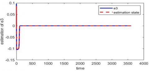
To obtain an accurate estimation for the time derivative of e2, the ACSMD was used, and the obtained result is shown in Figure 6 and compared with the actual value in the same figure. The results clarify the accuracy of the differentiation process with a smooth response. Moreover, the steady-state error is equal to or less than 4*10-5, which is the bound computed according to Remark (5).
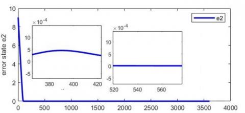
By using the estimated value of e3 to construct the sliding variable, the plot of s versus time is shown in Figure 7. As can be seen from this figure, the sliding variable is regulated in a few time interval and maintain its value within a bound not exceeds 0.05. As a result, the error goes asymptotically to zero as shown in Figure 8 and consequently the x2 follows the desired temperature.
Figure 6. Estimating the time derivative of e2
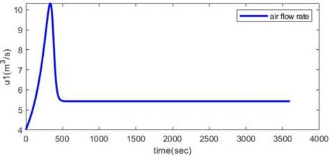
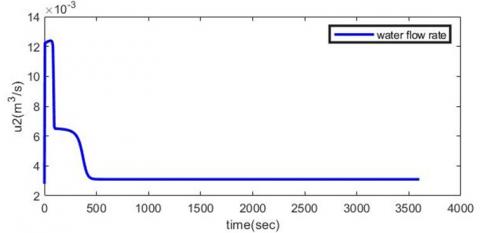
Figures 9 and 10 show that the control actions signal where the ASMC can effectively overcome the coupling control problem and compensate the first controller which is treated as an external disturbance.
The plots of the control signals are smooth due to replacing the [z]+ function by the approximation which is given in Eq. (29). Using the approximation in the control law eliminated the chattering phenomena with suitable values for β1 and β2 which were used to make the approximation as close as possible to the [z]+ function.
Figure 7. Sliding variable
Figure 8. Error state with 35%variation
Figure 9. Air flow rate with 35% variation
Figure 10. Water flow rate with 35% variation
6.3 HVAC system with 50% parameters variation
For more investigation of robustness and tracking of temperature and humidity ratios, different setpoints, and parameter variations are considered.
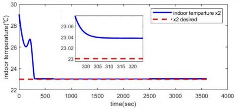
Figures 11 and 12 show the response of the humidity ration and indoor air temperature respectively with variation of 50% in parameters of the system. It is obvious that the proposed controllers can efficiently compensate the system parameters uncertainty. The obtained results reveal that the humidity ratio and the temperature follow the desired setpoints 0.0092kg H2O/kg dry air humidity ratio with ess=1.7*10-4 and 23℃ air temperature.
Figure 11. Time response humidity ratio with 50%variation
Figure 12. Time response temperature with 50%variation
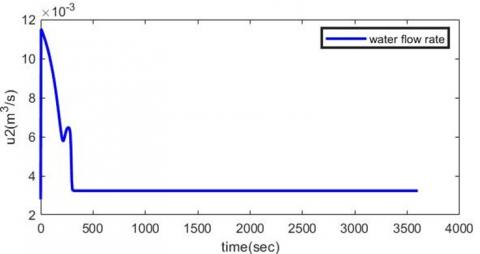
Since the gain of the first controller u1 depends on the upper bound of the variation, a higher value was obtained for this case than form the first case as can be deduced from Figure 13. This leads to a decrease in settling time and to a decrease in the ess (for humidity ratio control) as mentioned in Remark (4). The control action with 50% variation is shown in Figure 14, where the influence of the parameters variation and disturbance on the lower system appears in the reaching phase by increasing the settling time, however, eventually the value of the sliding variable does not exceed 0.05 as clarified in Figure 15. The results of the response of the two cases with different variation showed the ability of the proposed controllers in leading the state to track the desired value and achieve stability even when the system performance affected by the uncertainty and external disturbances.
Figure 13. Air flow rate with 50%variation
Figure 14. Water flow rate with 50%variation
Figure 15. Sliding variable with 50%variation
The HVAC system was presented which had MIMO. In this article, we proposed two control strategies to achieve robustness and desired to track. Firstly, the continuous feedback controls that choice is an essential issue for two reasons this is effective control to reject disturbance and it is differentiable which is needed in the designing of the second controller. Secondly, we proposed the adaptive sliding mode for the second controller, it is a proven choice in terms of reducing the system control efforts, minimizing gain values, and attenuation chattering than the classic SMC. Finally, to overcome uncertainty using ACSMD is an impressive choice that proved robustness and accurate result in estimating of error state. The proposed controls stability is verified using the Lyapunov theorem. The effectiveness of the proposed controllers was examined via the simulation results with 35%, and 50% variation in the system parameters and external disturbance. The controllers showed robustness and desirable performance by getting the desired thermal zone humidity ratio and temperature in the presence of uncertainty and external disturbance.
[1] Homod, R.Z., Gaeid, K.S., Dawood, S.M., Hatami, A., Sahari, K.S. (2020). Evaluation of energy-saving potential for optimal time response of HVAC control system in smart buildings. Applied Energy, 271: 115255. https://doi.org/10.1016/j.apenergy.2020.115255
[2] Fundamentals, A.H. (2005). American society of heating. Refrigerating and Air-Conditioning Engineers.
[3] Abdo-Allah, A., Iqbal, T., Pope, K. (2018). Modeling, analysis, and state feedback control design of a multizone HVAC system. Journal of Energy, Article ID: 4303580. https://doi.org/10.1155/2018/4303580
[4] Elnour, M., Meskin, N. (2017). Multi-zone HVAC control system design using feedback linearization. In 2017 5th International Conference on Control, Instrumentation, and Automation (ICCIA), pp. 249-254. https://doi.org/10.1109/icciautom.2017.8258687
[5] Afroz, Z., Shafiullah, G.M., Urmee, T., Higgins, G. (2018). Modeling techniques used in building HVAC control systems: A review. Renewable and Sustainable Energy Reviews, 83: 64-84. https://doi.org/10.1016/j.rser.2017.10.044
[6] Wallace, R.S. (1992). The harmonic impact of variable speed air conditioners on residential power distribution. In [Proceedings] APEC'92 Seventh Annual Applied Power Electronics Conference and Exposition, pp. 293-298. https://doi.org/10.1109/APEC.1992.228399
[7] Jahedi, G., Ardehali, M.M. (2012). Wavelet based artificial neural network applied for energy efficiency enhancement of decoupled HVAC system. Energy Conversion and Management, 54(1): 47-56. https://doi.org/10.1016/j.enconman.2011.10.005
[8] Moradi, H., Saffar-Avval, M., Bakhtiari-Nejad, F. (2011). Nonlinear multivariable control and performance analysis of an air-handling unit. Energy and Buildings, 43(4): 805-813. https://doi.org/10.1016/j.enbuild.2010.11.022
[9] Kang, C.S., Park, J.I., Park, M., Baek, J. (2014). Novel modeling and control strategies for a HVAC system including carbon dioxide control. Energies, 7(6): 3599-3617. https://doi.org/10.3390/en7063599
[10] Azarbani, A., Abbasi, R. (2019). Optimal state estimation of air handling unit system without humidity sensor using unscented kalman filter. In 2019 6th International Conference on Control, Instrumentation and Automation (ICCIA), pp. 1-6. https://doi.org/10.1109/ICCIA49288.2019.9030871
[11] Liavoli, F.B., Fakharian, A. (2019). Sub-optimal observer-based controller design using the state dependent riccati equation approach for air-handling unit. In 2019 27th Iranian Conference on Electrical Engineering (ICEE), pp. 991-996. https://doi.org/10.1109/IranianCEE.2019.8786630
[12] Shah, Z.A., Sindi, H.F., Ul-Haq, A., Ali, M.A. (2020). Fuzzy logic-based direct load control scheme for air conditioning load to reduce energy consumption. IEEE Access, 8: 117413-117427. https://doi.org/10.1109/ACCESS.2020.3005054
[13] Ganchev, I., Taneva, A., Kutryanski, K., Petrov, M. (2019). Decoupling fuzzy-neural temperature and humidity control in HVAC systems. IFAC-PapersOnLine, 52(25): 299-304. https://doi.org/10.1016/j.ifacol.2019.12.539
[14] Liavoli, F.B., Shadi, R., Fakharian, A. (2021). Multivariable nonlinear model predictive controller design for air-handling unit with single zone in variable air volume. In 2021 7th International Conference on Control, Instrumentation and Automation (ICCIA), pp. 1-6. https://doi.org/10.1109/ICCIA52082.2021.9403555
[15] Utki, V.I. (1992). Sliding Modes in Control and Optimizations. Springer-Verlag Berlin, Heidelberg. https://doi.org/1007/978-3-642-84379-2
[16] Utkin, V.I. (1978). Sliding Modes and Their Applications in Variable Structure Systems. Mir, Moscow.
[17] Shah, A., Huang, D., Chen, Y., Kang, X., Qin, N. (2017). Robust sliding mode control of air handling unit for energy efficiency enhancement. Energies, 10(11): 1815. https://doi.org/10.3390/en10111815
[18] Shah, A., Huang, D., Huang, T., Farid, U. (2018). Optimization of buildingsenergy consumption by designing sliding mode control for multizone VAV air conditioning systems. Energies, 11(11): 2911. https://doi.org/10.3390/en11112911
[19] Utkin, V.I., Poznyak, A.S. (2013). Adaptive sliding mode control with application to super-twist algorithm: Equivalent control method. Automatica, 49(1): 39-47. https://doi.org/10.1016/j.automatica.2012.09.008
[20] Plestan, F., Shtessel, Y., Bregeault, V., Poznyak, A. (2010). New methodologies for adaptive sliding mode control. International Journal of Control, 83(9): 1907-1919. https://doi.org/10.1080/00207179.2010.501385
[21] Al-samarraie, S.A., Ali, L.F. (2018). Output feedback adaptive sliding mode control design for a plate heat exchanger. Al-Nahrain Journal for Engineering Sciences, 21(4): 549-555. http://doi.org/10.29194/NJES.21040532
[22] Afram, A., Janabi-Sharifi, F. (2014). Theory and applications of HVAC control systems–A review of model predictive control (MPC). Building and Environment, 72: 343-355. https://doi.org/10.1016/j.buildenv.2013.11.016
[23] Arguello-Serrano, B., Velez-Reyes, M. (1999). Nonlinear control of a heating, ventilating, and air conditioning system with thermal load estimation. IEEE Transactions on Control Systems Technology, 7(1): 56-63. https://doi.org/10.1109/87.736752
[24] Utkin, V., Guldner, J., Shi, J. (2009). Sliding Mode Control in Electro-Mechanical Systems. CRC Press. https://doi.org/10.1201/9781420065619
[25] Shtessel, Y., Edwards, C., Fridman, L., Levant, A. (2014). Sliding Mode Control and Observation. New York: Springer New York. https://doi.org/10.1007/978-0-8176-4893-0
[26] AL-Samarraie, S.A., Mahdi, S.M., Ridha, T.M.M., Mishary, M.H. (2015). Sliding mode control for electro-hydraulic servo system. Iraqi J Comput Commun Control Syst Eng, 15(3): 1-10.
[27] Humaidi, A.J., Hameed, A.H., Ibraheem, I.K. (2019). Design and performance study of two sliding mode backstepping control schemes for roll channel of delta wing aircraft. In 2019 6th International Conference on Control, Decision and Information Technologies (CoDIT), pp. 1215-1220. https://doi.org/10.1109/CoDIT.2019.8820315
[28] Tavoosi, J. (2020). A new type-2 fuzzy sliding mode control for longitudinal aerodynamic parameters of a commercial aircraft. Journal Européen des Systèmes Automatisés, 53(4): 479-485. https://doi.org/10.18280/jesa.530405
[29] Utkin, V.I., Poznyak, A.S. (2013). Adaptive sliding mode control. In Advances in Sliding Mode Control, pp. 21-53.
[30] Tohma, D.H., Hamoudi, A.K. (2021). Design of adaptive sliding mode controller for uncertain pendulum system. Eng. Technol. J, 39: 355-369. http://dx.doi.org/10.30684/etj.v39i3A.1546
[31] Majeed, H.S., Kadhim, S.K., Jaber, A.A. (2022). Design of a sliding mode controller for a prosthetic human hand’s finger. Engineering and Technology Journal, 40(1): 257-266. http://dx.doi.org/10.30684/etj.v40i1.1943
[32] Humaidi, A.J., Sadiq, M.E., Abdulkareem, A.I., Ibraheem, I.K., Azar, A.T. (2021). Adaptive backstepping sliding mode control design for vibration suppression of earth-quaked building supported by magneto-rheological damper. Journal of Low Frequency Noise, Vibration and Active Control. https://doi.org/10.1177/14613484211064659
[33] Al-Samarraie, S.A. (2018). Variable structure control design for a magnetic levitation system. Journal of Engineering, 24(12): 84-103. https://doi.org/10.31026/j.eng.2018.12.08
[34] AL-Samarraie, S.A. (2018). A chattering free sliding mode observer with application to DC motor speed control. In 2018 Third Scientific Conference of Electrical Engineering (SCEE), pp. 259-264. https://doi.org/10.1109/SCEE.2018.8684128
[35] Rakan, A.B., Ridha T.M., AL-Samarraie, S.A. (2022). Artificial pancreas: Avoiding hyperglycemia and hypoglycemia for type one diabetes. Engineering and Information Technology, 12(1): 194-201. http://dx.doi.org/10.18517/ijaseit.12.1.15106