Full State Feedback H-Infinity Controller Design for Nonlinear Systems

Nonlinear systems are considered the most important topic in control theory over the last few decades. They are of great importance due to their applications in science and engineering [1]. Nonlinear phenomena typically represent a real-world system's behavior. Due to the significant uncertainty and nonlinearity of these systems, it is challenging to keep appropriate stability margins and required performance characteristics for closed-loop systems. So, a robust control methods are needed to design controllers for nonlinear systems that meeting the stabilization and required performance in facing the uncertainties and nonlinearities [2].

The most frequent and effective strategy in robust control theory for rejecting disturbances and compensating nonlinearities and uncertainties in the system is the H-infinity control. It provides a strong performance and stabilization [3-6]. The development of robust feedback controllers is a key challenge in control theory. Tracking asymptotically and robustness despite system disturbances and uncertainties care tasks that such controllers may undertake [7]. The feedback control theory entails numerous feedback structure choices and multiple feedback loops. A state feedback control is a kind of feedback control in which all of the system states be available for feedback [8].

Previous research has focused on a variety of design strategies for robust feedback control, like the design of H-infinity state feedback control depending on the model that is nearly linearized [9, 10], the robust feedback linearization for nonlinear processes control based on Lyapunove theory [11], H-infinity loop-shaping approach [12, 13], a robust control method on the basis of linear and bilinear matrix inequalities, (LMIs)&(BMIs) [14, 15].

All of the studies mentioned above presented relatively complex algorithm for designing a controller for nonlinear systems and are specific to the type of system, this is what prompted us to do this study, which suggests simple and more general algorithm.

In this paper, a full state feedback H-infinity controller is designed to stabilize the nonlinear systems and satisfy a desirable performance. The Black Hole optimization (BHO) method is employed to obtain the optimum parameters for the suggested nonlinear controller. The proposed controller design in this paper can effectively compensate the nonlinear systems with constant coefficients.

The structure of the paper is as follows: in “BLACK HOLE OPTIMIZATION (BHO)” section the optimization method (BHO) is explained. In “CONTROLLER DESIGN” section the formulation of the full state feedback H∞ nonlinear control problem for the nonlinear system is provided. In “CONTROLLER PARAMETERS TUNING” section the parameters of the proposed controller that will be tuned by the BHO to obtaining the optimal values for them were reviewed. In “ILLUSTRATIVE EXAMPLES” section two kinds of nonlinear systems are presented as case studies to demonstrate the effectiveness of the proposed controller. In “CONCLUSION” section concluding remarks are stated.

In this section, the design procedure of the proposed controller for the systems that have the form [20, 21]:

$\dot{x}=A x+B_1 d(t)+B_2 u(t)\\

e(t)=C_1 x+D_{12} u(t)\\

y=C_2 x$         (3)

where, $x \in \mathcal{R}^n$ is the system state, $d(t) \in \mathcal{R}^m$ is the exogenous disturbance, $u(t) \in \mathcal{R}^l$ is the control input, $e(t) \in \mathcal{R}^q$ is the controlled output, $y \in \mathcal{R}^p$ is the measured output, which is the state vector, assumed to be available for feedback, $A \in \mathcal{R}^{n \times n}$, $B_1 \in \mathcal{R}^{n \times m}$ and $B_2 \in \mathcal{R}^{n \times l}$, $C_1 \in \mathcal{R}^{q \times n}$ is a weight matrix of the system state control, $D_{12} \in \mathcal{R}^{q \times l}$ is a weight matrix of control input regulation, $C_2 \in \mathcal{R}^{p \times n}$ is the output weight matrix.

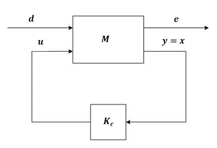
The standard configuration of the full state feedback H-infinity control is as shown in Figure 1, where M represents the augmented plant matrix [21]:

$M=\left[\begin{array}{ccc}A & B_1 & B_2 \\ C_1 & D_{11} & D_{12} \\ C_2 & D_{21} & D_{22}\end{array}\right]$          (4)

1.png

Figure 1. Full state feedback H-infinity control structure

As we need to design a full state feedback H-infinity control, all system states must be available for feedback. This implies that C₂=I.D₁₁, D₂₁ and D₂₂=0. So the augmented plant matrix M becomes:

$M=\left[\begin{array}{ccc}A & B_1 & B_2 \\ C_1 & 0 & D_{12} \\ I & 0 & 0\end{array}\right]$       (5)

The following assumptions are required for the proposed controller's design:

(1) The pairs (A, B₁) and (A, B₂) are stabilizable.

(2) The pair (C₁, A) is detectable.

(3) $C_1^T D_{12}=0$ and $D_{12}^T D_{12}=I$.

It is worth to mention that to control a nonlinear system in this procedure, it should be converted to the configuration shown in Eq. (3) using a state variable transformation method. This transformation makes the nonlinear terms and uncertainties (bad terms) arranged in the same channel in which the control law $u$ affects (satisfying the matching condition). In this case the controller can compensate the bad terms. The appropriate transformation for this object is the diffeomorphism mapping: $T: \mathcal{D} \rightarrow \mathcal{R}^n$ which transforms the system from x-space to z-space [22].

$\mathrm{z}=T(x)$       (6)

The map T must be invertible, such that

$x=T^{-1}(z)$        (7)

The transformed system’s origin point in z-space is the same as the original system [22]:

T(0)=0          (8)

This mapping converts the nonlinear system to the following structure [8]:

$\dot{z}=A z+B_1 d(t)+B_2 u(t)$        (9)

The control problem is to find the optimal control law u^*, which is a function of states, that makes the system internally stable by ensuring the infinite norm of the closed-loop transfer function (T_ed) which should be less than a given value of γ as [20]:

$\left\|T_{e d}(s)\right\|_{\infty}<\gamma$       (10)

where, γ represents the upper bound in the disturbance and uncertainty magnitude that can be exterminated by the control signal. The condition in Eq. (10) implies that [21]:

$\begin{array}{rr}\text { inf } & \sup \\ u & d\end{array}(u, d)<\infty$        (11)

where

$J(u, d)=\int_0^{\infty}\left(e^T e-\gamma^2 d^T d\right) d t$       (12)

The disturbance d(t) tries to maximize the cost function J(t) while the control signal u(t) tries to minimize it. Therefore, the physical meaning of this relation is that the control signal and the disturbance compete to each other within infimum (inf) and supremum (sup).

Let the optimal control and worst-case disturbance have the following structure [19]:

$d(t)=K_d x(t)$        (13)

and

$u(t)=K_c x(t)$        (14)

Substituting Eq. (14) in Eq. (3), yields:

$e(t)=\left(C_1+D_{12} k_c\right) x(t)$          (15)

Using assumption 3 gives:

$e^T e=\boldsymbol{X}^T\left(C_1^T C_1+K_c^T K_c\right) \boldsymbol{X}$         (16)

Therefore,

$J=\int_0^{\infty} x^T\left(C_1^T C_1+K_c^T K_c-\gamma^2 K_d^T K_d\right) x d t$           (17)

Substituting Eq. (15) and Eq. (16) in Eq. (3), yields:

$\dot{x}=\left(A+B_1 K_d+B_2 K_c\right) x$          (18)

With the performance index in Eq. (17), let:

$Q=\left(C_1^T C_1+K_c^T K_c-\gamma^2 K_d^T K_d\right)$          (19)

where, Q must be positive definite matrix. The system in Eq. (18) is assumed to be stable by this optimal control law. Under this assumption, let us set:

$V(x)=x^T P x$        (20)

$\dot{V}(x)=-x^T Q x$         (21)

where, V(x) is positive definite Lyapunov quadratic function. To find the optimal cost function, Eq. (19) will be substituted in Eq. (21) to get:

$\dot{V}(x)=-x^T\left(C_1^T C_1+K_c^T K_c-\gamma^2 K_d^T K_d\right) x$          (22)

$x^T\left(C_1^T C_1+K_c^T K_c-\gamma^2 K_d^T K_d\right) x=-\frac{d}{d t} x^T P x$        (23)

Integrating both sides of Eq. (23) from 0 to $\infty$ yields:

$\begin{aligned} \int_0^{\infty} x^T\left(C_1^T C_1+K_c^T\right.&\left.K_c-\gamma^2 K_d^T K_d\right) x d t=\int_0^{\infty}-\frac{d}{d t} x^T P x d t \end{aligned}$        (24)

$J=-x(\infty)^T P x(\infty)-\left(-x(0)^T P x(0)\right)$        (25)

Since the system in Eq. (18) must be stable by the control law, $x(\infty)=0$. Therefore, the optimal cost function is:

$J^*=-x(0)^T P x(0)$         (26)

The positive definite matrix P represents the solution of the following Lyapunov equation:

$\left(A+B_1 K_d+B_2 K_c\right)^T P+P\left(A+B_1 K_d+B_2 K_c\right)=-Q$          (27)

$\left(A+B_1 K_d+B_2 K_c\right)^T P+P\left(A+B_1 K_d+B_2 K_c\right)=-\left(C_1^T C_1+K_c^T K_c-\gamma^2 K_d^T K_d\right)$        (28)

$\left(A+B_1 K_d+B_2 K_c\right)^T P+P\left(A+B_1 K_d+B_2 K_c\right)+\left(C_1^T C_1+K_c^T K_c-\gamma^2 K_d^T K_d\right)=0$       (29)

Now, to find the optimal control law we must derive Eq. (29) w.r.t. K_c and make $\partial P / \partial K_{c_{i j}}=0$, we get:

$K_c=-B_2^T P$         (30)

As a result,

$u^*=K_c x=-B_2^T P x$         (31)

By the same way, we can find the applied worst-case disturbance by deriving the Lyapunov equation w.r.t. K_d and make $\partial P / \partial K_{d_{i j}}=0$, we get:

$K_d=\frac{1}{\gamma^2} B_1^T P$        (32)

and

$d^*=K_d x=\frac{1}{\gamma^2} B_1^T P x$         (33)

The Lyapunov equation at the optimal control case and worst-case disturbance is:

$P A+A^T P+C_1^T C_1-P\left(B_2 B_2^T-\frac{1}{\gamma^2} B_1 B_1^T\right) P=0$       (34)

This equation is known as the H-infinity algebraic riccati equation.

The condition $\left\|T_{e d}(s)\right\|_{\infty}<\gamma$ is satisfied and provided:

(1) $u^*=K_c x=-B_2^T P x$.

(2) P>0.

The matrix A+B₁K_d+B₂K_c is stable and implies that the matrix A+B₂K_c is asymptotically stable.

Two nonlinear system examples are offered in this section as case studies to demonstrate the usefulness of the proposed controller. The time responses of the nonlinear system without and with the proposed controller are presented to demonstrate the effectiveness of the proposed controller. In example 1, the matching condition is satisfied in the state equations of the nonlinear system (the nonlinear terms and the control law are located in the same channel). In example 2, the matching condition is not satisfied (the nonlinear terms and the control law are located in different channels).

5.1 Example 1

The nonlinear system to be controlled is:

$\dot{x}_1=x_2\\

\dot{x}_2=\sin x_1-u \cos x_1\\

y=x_1$       (35)

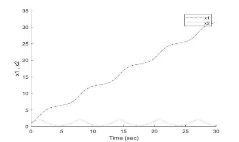
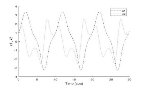
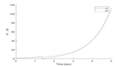
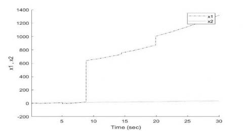
Figures 3 and 4 show the nonlinear system's open-loop and closed-loop time response properties before applying the proposed controller. It is clear that the system is unstable in open-loop and critical stable in closed loop, so it is necessary to design a controller to stabilize the system and achieve the required performance. For this system, there is no need to utilize the diffeomorphism mapping because all nonlinear terms are located in the same channel of control u (matching condition is satisfied). It is noted from system’s equation Eq. (35) that the coefficient of u is variable and nonlinear term of the state x₁. Therefore, to make the system’s equation (Eq. (35)) in the standard controllable form as Eq. (3), the following steps are required:

$v=-u \cos x_1$       (36)

3.jpg

Figure 3. Time response for closed-loop system

4.jpg

Figure 4. Time response for open-loop system

where, υ represents the virtual linear state feedback controller, which is:

$v=K_C x=K_1 x_1+K_2 x_2$        (37)

Then the actual controller u is:

$u=-\frac{v}{\cos x_1}=-\frac{K_c x}{\cos x_1}=\frac{-K_1 x_1-K_2 x_2}{\cos x_1}$       (38)

The resulting system state equation is:

$\dot{x}(t)=\left[\begin{array}{ll}0 & 1 \\ 0 & 0\end{array}\right] x(t)+\left[\begin{array}{l}0 \\ 1\end{array}\right] d(t)+\left[\begin{array}{l}0 \\ 1\end{array}\right] v(t)$        (39)

where,

$d(t)=\sin x_1$        (40)

The BHO algorithm was then utilized to find the optimal control law. Table 1 displays the optimization settings for the BHO algorithm. As well as, Table 2 displays the optimal values and bounds of the optimized parameters.

Table 1. The settings of BHO algorithm (example 1)

Table 2. The optimized parameters' bounds and optimal values (example 1)

Subsequently, the H-infinity algebraic equation (Eq. (34)) will be solved with the obtained optimal values to obtain the stabilizing positive definite matrix P as follows:

$P=10^3\left[\begin{array}{ll}2.1911 & 0.2400 \\ 0.2400 & 0.0526\end{array}\right]$         (41)

Then, the gain matrix of the state feedback controller has been determined using Eq. (30) as seen below:

$K_c=\left[\begin{array}{ll}-240.0397 & -52.5944\end{array}\right]$         (42)

Thus, the control law becomes:

$u=\frac{240.0397 x_1+52.5944 x_2}{\cos x_1}$       (43)

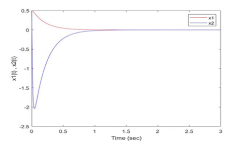
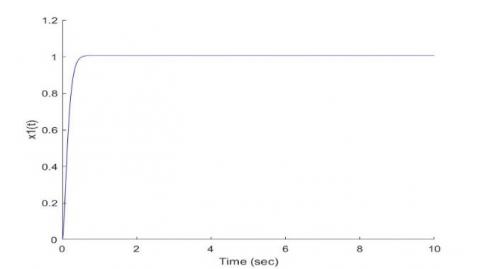
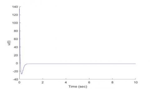
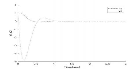
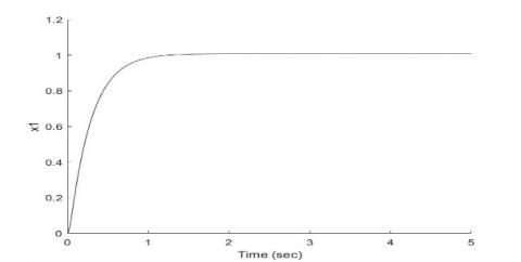
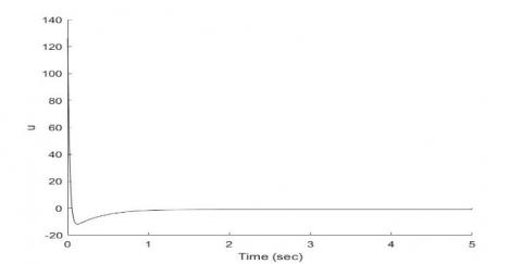
Figures 5 and 6 show the time response of the nonlinear system after applying the proposed controller to the system and achieving the stabilization and tracking for a unit step reference input. Figure 7 shows the behavior of the control signal. It is shown that the proposed controller can effectively stabilize the nonlinear system with a desirable performance.

5.png

Figure 5. Stabilization properties of nonlinear system states

6.jpg

Figure 6. Tracking properties

7.jpg

Figure 7. The resulting control action

5.2 Example 2

Consider the nonlinear system to be controlled:

$\dot{x}_1=\tan x_1+x_2\\

\dot{x}_2=x_1+u\\

y=x_1$         (44)

8.jpg

Figure 8. Time response for open-loop system

9.jpg

Figure 9. Time response for closed-loop system

Figures 8 and 9 show the nonlinear system’s open-loop and closed-loop time response properties before applying the suggested controller.

It is clear that the system is unstable in open-loop and closed loop, so it is necessary to design a controller to stabilize the system and achieve the required performance. It is noticed that the nonlinear term (tanx₁) isn’t located in the same channel that control signal u effects (matching condition not satisfied), so the diffeomorphism mapping of Eq. (6) is necessary to transform the nonlinear system into the standard controllable form as in Eq. (9). To carry out the mapping, the following state variable transformation will apply:

$z_1(t)=x_1(t), z_2(t)=\dot{z}_1(t)=\dot{x}_1(t)=\tan x_1+x_2$        (45)

Thus, the transformed state equation becomes:

$\dot{z}_1(t)=z_2(t)\\

\dot{z}_2(t)=z_1+d(t)+u(t)$      (46)

where, $d(t)=z_2 \sec ^2 z_1$.

Then the system in z-space becomes:

$\left[\begin{array}{l}\dot{z}_1(t) \\ \dot{z}_2(t)\end{array}\right]=\left[\begin{array}{ll}0 & 1 \\ 1 & 0\end{array}\right]\left[\begin{array}{l}z_1(t) \\ z_2(t)\end{array}\right]+\left[\begin{array}{l}0 \\ 1\end{array}\right] d(t)+\left[\begin{array}{l}0 \\ 1\end{array}\right] u(t)$        (47)

The BHO algorithm was then utilized to find the optimal control law. Table 3 shows the settings for optimization of the BHO algorithm. As well as, Table 4 shows the bounds of the optimized parameter and their optimal values.

Table 3. The settings of BHO algorithm (example 2)

Table 4. The optimized parameters' bounds and optimal values (example 2)

Subsequently, the H-infinity algebraic equation (Eq. (34)) will be solved with the obtained optimal values to obtain the stabilizing positive definite matrix P as follows:

$P=10^3\left[\begin{array}{cc}0.7943 & 0.1259 \\ 0.1259 & 0.038\end{array}\right]$        (48)

Then, the gain matrix of the state feedback controller has been determined using Eq. (30) as seen below:

$K_c=\left[\begin{array}{ll}-125.9200 & -38.0930\end{array}\right]$       (49)

Thus, the optimal control law in z-space becomes:

$u=-125.92 z_1-38.093 z_2$       (50)

Now, the control law will be converted from z-space to x-space:

$u=-125.92 x_1-38.093 \tan x_1-38.093 x_2$       (51)

Figures 10 and 11 show that the proposed controller was succussed in achieving stabilization and tracking performance, with minimum tracking error and rapid convergence to the reference line, for the nonlinear system despite the presence of disturbance. Figure 12 shows the behavior of the implemented control action which is admissible.

10.jpg

Figure 10. Stabilization properties of nonlinear system states

11.jpg

Figure 11. Tracking properties

12.jpg

Figure 12. The resulting control action