Zoubir Gadouche | Cheikh Belfedal | Tayeb Allaoui* | Mouloud Denai | Mohammed Bey
© 2022 IIETA. This article is published by IIETA and is licensed under the CC BY 4.0 license (http://creativecommons.org/licenses/by/4.0/).
OPEN ACCESS
The paper suggests a novel DPC approach to ameliorate the management and HRES “hybrid renewable energy system” control composed of photovoltaic and wind systems. In the conventional DPC technique, the “switching table” is founded on a “hysteresis comparator”, which poses the problem of fluctuations on the HRES various output variables. The approach proposed here is based on an FLC and shown to diminish the ripples in the “active” and “reactive” powers waveforms. The comprehensive HRES and the advised “control schemes” are implemented using “MATLAB/Simulink” and the results indicate that the advised method had preferable performance over the conventional DPC.
photovoltaic, wind turbine (WT), hybrid energy conversion, direct power control (DPC), fuzzy logic controller (FLC)
Today and despite the great development and exploitation of renewable energy sources, according to the different statistics published in the reviews, the integration of this type of energy in various energy sectors, does not exceed 20% compared to the global demand for electrical energy [1]. However, the major problem is the irregular nature of the energy supply. To overcome this disadvantage, it is often necessary to combine several energy sources enabling greater energy production and a better regularity. Wind energy combined with solar photovoltaic has been the focus of several research investigations. In the latest signal processing technology have enabled the realization of additional control structures equivalent to “vector control” technology that ensures both system robustness and higher power quality [2]. The recent steps generality during this direction are those classified under the terms DTC “direct torque control” and DPC. These control concepts have certainly evolved in the last few years, aiming to improve aspects such as minimizing the influence of machine parameters [3].
The major disadvantages of this control strategy are the oscillations in the power and generation of harmonic current due to the variable switching frequency [4-7].
In this paper, it is proposed to apply a new DPC technique to control the power flow in the wind-solar photovoltaic HES. This approach uses a different switching table structure and the selection control vector is based on the application of the fuzzy rules. The reference pursuit errors of “active” and “reactive” powers, regenerate into “fuzzy variables”, are used to select the suitable “control vector” [8].
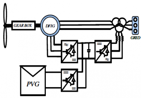
Figure 1 clarifies the proposed configuration of the system and its integration to the grid via the RSC “rotor side converter” of the WT and GSC “grid side converter”.
This control scheme is mainly founded on the choice of the “voltage vector” such that the errors among the reference and measured quantities are decreased and maintained among the boundaries of the “hysteresis bands” [4, 9-11]. The principal qualities of this control shape are progressed responsiveness speed and low reliance on the machine parameters [12].
The final paper is prepared as follows: division 2 explains the modelling of the proposed HRES. Division 3 explains the Photovoltaic system control. Division 4 explains the classical control techniques proposed in this paper for the HRES. The F-DPC “fuzzy DPC” based control system is offered in division 5. The simulation results are offered in Division 6 and finally, discussions and conclusions are approached in division 7.
Figure 1. Hybrid energy system global schema
Figure 1 demonstrates the “HRES” proposed configuration and its integration to the grid via RSC of the WT and GSC.
2.1 Modeling of the Wind Energy System (WES)
2.1.1 WT model
The WT transform the “wind energy” into “mechanical energy”. "Wind power" is explained as follows [13]:
$P_V=\frac{\rho \cdot S \cdot v^3}{2}$ (1)
$P_{\text {aer }}=C_p \cdot P_v=C_p(\lambda, \beta) \cdot \frac{\rho \cdot S \cdot v_v^3}{2}$ (2)
$\lambda=\frac{R . \Omega_{\text {turbine }}}{v_v}$ (3)
where, “Tip speed ratio” is λ, “turbine mechanical speed” is $\Omega_{\text {turbine }}$, “wind speed” is Vv, and “turbine radius” is R.
The power coefficient depicts the WT aerodynamic efficiency, it is determined as follows:
$C_p=0.5176\left(\frac{116}{\lambda_i}-0.4 \beta\right) \exp ^{\left(\frac{21}{\lambda_i}\right)}+0.0068 \lambda$ (4)
with:
$\frac{1}{\lambda_i}=\frac{1}{\lambda+0.008 \beta}-\frac{0.035}{1+\beta^3}$ (5)
The relationship between Cp and λ for the given values of the blade pitch angle is represented by Eq. (2).
From this power, the wind torque is determined by:
$T_{a e r}=\frac{P_{a e r}}{\Omega_{\text {turbine }}}=C_p \cdot \frac{\rho \cdot S \cdot v^3}{2} \cdot \frac{1}{\Omega_{\text {turbine }}}$ (6)
The mechanical speed can be determined using the following mechanical equation:
$J . \frac{d \Omega_{m e c}}{d t}=T_{m e c}$ (7)
where, Tmec is “torque” exercised to the “generator rotor” and J is “total inertia” that take shape on the “generator rotor” presented by:
$J=\frac{J_{\text {turbine }}}{G^2}+J_g$ (8)
The Tmec “mechanical torque” takes the Tem “electromagnetic torque” into account developed by the generator, the Tvis “viscous friction torque”, and the Tg “torque from the multiplier”.
$T_{\text {mec }}=T_g-T_{e m}-T_{v i s}$ (9)
2.1.2 Wind generator model
DFIG “mathematical model” is presented by system of five “differential equations”, in (d,q) “Park reference frame” [13].
$\left\{\begin{array}{l}\frac{d \varphi_{s d}}{d t}=\frac{-1}{\sigma T_s} \varphi_{s d}+\omega_s \varphi_{s q}+\frac{M_{s r}}{\sigma T_s L_r} \varphi_{r d}+v_{s d} \\ \frac{d \varphi_{s q}}{d t}=\frac{-1}{\sigma T_s} \varphi_{s q}-\omega_s \varphi_{s d}+\frac{M_{s r}}{\sigma T_s L_r} \varphi_{r q}+v_{s q} \\ \frac{d \varphi_{r d}}{d t}=\frac{-1}{\sigma T_r} \varphi_{r d}+\omega_r \varphi_{r q}+\frac{M_{s r}}{\sigma T_r L_r} \varphi_{s d}+v_{r d} \\ \frac{d \varphi_{r q}}{d t}=\frac{-1}{\sigma T_r} \varphi_{r q}+\omega_r \varphi_{r d}+\frac{M_{s r}}{\sigma T_r L_r} \varphi_{s q}+v_{r q}\end{array}\right.$ (10)
And using the "torque" equation [13]:
$T_{e m}=p \frac{1-\sigma}{\sigma M_{s r}}\left(\varphi_{r d} \varphi_{s q}-\varphi_{r q} \varphi_{s d}\right)$ (11)
2.2 Photovoltaic Energy System (PES) model
The photovoltaic cell equivalent circuit is the one-diode model. The two resistors Rs and Rp are introduced to model the cell defects [14].
The circuit operates as a generator can thus be constituted by an equations system given from “Kirchhoff's laws”. The “I-V” characteristic of an ideal photovoltaic cell described mathematically by the basic equation of semiconductor theory is as follows [14].
$I=I_{p v}-I_d-I_p$ (12)
The current is delivered to a “P-N junction” in silicon, and the voltage at its terminals is given by:
$I_d=I_o\left[\exp \left(\frac{q\left(V+R_s I\right)}{a K T}\right)-1\right]$ (13)
where, V is the voltage across its terminals. The current Ip is presented by the following equation:
$I_p=\frac{V+R_s I}{R_p}$ (14)
Substituting $I_d$ and $I_q$ in Eq. (12) gives:
$I=I_{p v}-I_o\left[\exp \left(\frac{q\left(V+R_s I\right)}{a K T}\right)-1\right]-\frac{V+R_s I}{R_p}$ (15)
Assume that $R_p \gg R_s$ hence $I_p \approx 0$ which leads to:
$I=I_{p v}-I_o\left[\exp \left(\frac{q\left(V+R_s I\right.}{a K T}\right)-1\right]$ (16)
$I=I_{p v, \text { cell }}-I_{o, \text { cell }}\left[\exp \left(\frac{q V}{a K T}\right)-1\right]$ (17)
The “current” and “voltage” relationship in a PVG “photovoltaic generator”, several cells consisting associated in "series and parallel" is presented by the subsequent equation [15]:
$I=N_p \cdot I_{p v}-N_p \cdot I_o\left[\exp \left(\frac{q\left(V+\frac{N_s}{N_p} R_s \cdot I\right)}{N_s \cdot a \cdot K \cdot T}\right)-1\right]$ (18)
2.3 DC bus model
The two energy sources are coupled via a “DC bus”, as presented in Figure 2.
Figure 2. DC bus representation
The DC bus voltage is given by:
$V_{d c}=\frac{1}{C} \cdot \int_0^t I_c \cdot d t$ (19)
The current in the capacitor is from a node from which the circulating current is modulated by the hybrid source and the GSC.
$I_c=I-I_{G S C}=\left(I_{d f i g_{-} \text {rotor }}+I_{p v}\right)-I_{G S C}$ (20)
2.4 Grid converter model
For system modelling, the converter is sectioned into 3 parts: the “AC side”, the discontinuous part formed by the “switches” and the “DC side” [16].
The “switches” are complementary; their status is determined by the following function [16]:
$S_j=\left\{\begin{array}{l}1, \bar{S}_j=0 \\ 0, \bar{S}_j=1\end{array}\right.$ (21)
The “input phase voltages” and the “output current” enable to write in relation to Sj, Vdc and the “input currents”.
$C \frac{d V_{d c}}{d t}=\left(S_a i_a+S_b i_b+S_c i_c\right)-I$ (22)
With
$I_c=S_a i_a+S_b i_b+S_c i_c$ (23)
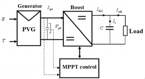
“MPPT control” permits the “maximum power” elicitation of the “PVG” Under the changing weather and load conditions. The principle of control is based on the “duty cycle D” automatic alteration of the “DC-DC boost converter” so as to maximize the PVG "output power" (Figure 3) [17].
The MPPT method employed here is the Perturb and Observe (P&O). The inputs are the voltage and current of the solar panel, and the output is either the voltage reference or the duty cycle. As its name indicates the method of (P&O), operates by the disturbance of the system either by increasing or decreasing the operating voltage and observing its impact on panel output power [18].
Figure 3. Block diagram of the PV system by an MPPT control
The DPC concept is founded on the “voltage vectors” selection, predefined in a “switching table”, applied to the 3 phase “PWM converter”. These “voltage vectors” represent sequences of “switching states” of the converter switches “Sa, Sb, Sc”. The selection is made on the fundamental of the errors (Sp, Sq) between the references (P*, Q*) and the actual values (P, Q) of the “active power” and “reactive power”, as well as on the “angular position θ”of the flux vector for RSC and the “grid voltage vector” for GSC [2, 10]. One of the controls is simpler and robust than “vector control” which is the DPC strategy on account of the lower dependence of DFIG parameters.
4.1 “Wind Energy System” control using C-DPC
4.1.1 Switching table elaboration powers estimation
Rather than measuring power on the line, we capture the “rotor currents” and estimate “Ps” and “Qs”. This manner grants early the "powers control" of the stator windings.
Recall that the “DPC control” will be based on the simplified DFIG model, i.e. that determined by ignoring the stator phase resistance. We can find the relationship of “Ps” and “Qs” based on two constituents of the rotor flux in the reference repository (αr, βr).
The powers are estimated using the subsequent relationships [18]:
$\left\{\begin{array}{l}P_s=-\frac{3}{2} \frac{L_m}{\sigma L_s L_r} V_s \varphi_{r \beta} \\ Q_s=\frac{3}{2} V_s\left(\frac{1}{\sigma L_s} \psi_s-\frac{L_m}{\sigma L_s L_r} \varphi_{r \alpha}\right)\end{array}\right.$ (24)
With:
$\left\{\begin{array}{l}\varphi_{r \alpha}=\sigma L_r i_{r \alpha}+\frac{L_m}{L_s} \psi_s \\ \varphi_{r \beta}=\sigma L_r i_{r \beta} \\ \left|\bar{\psi}_s\right|=\frac{\left|\bar{V}_s\right|}{\omega_s}\end{array}\right.$ (25)
Input the angle δ amid the stator and rotor flux vector, then “Ps” and “Qs” become:
$\left\{\begin{array}{l}P_s=-\frac{3}{2} \frac{L_m}{\sigma L_s L_r} \omega_s\left|\psi_s\right|\left|\psi_r\right| \sin \delta \\ Q_s=\frac{3}{2} \frac{\omega_s}{\sigma L_s}\left|\psi_s\right|\left(\frac{L_m}{L_r}\left|\psi_r\right| \cos \delta-\left|\psi_s\right|\right)\end{array}\right.$ (26)
4.1.2 Switching table elaboration
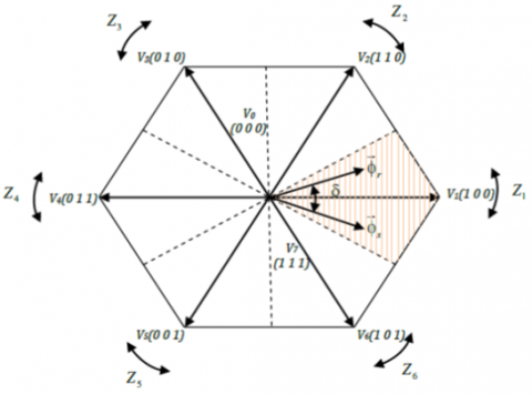
To designate the optimal rotor “voltage vector”, it is required to define the “rotor flux” related position in the “six sextants”. A “3-phase inverter” with two “voltage levels” can create eight various combinations and eight combinations generate eight "voltage vectors" that ability to use for the DFIG rotor terminals.
There are six “active vectors” and two “null vectors”. The spatial positions of the “active voltage vectors” in the (αr, βr) plane are displayed in Figure 4.
The "complex plane" partition into "six sectors" SEC $(\mathrm{i}=1, \ldots, 6)$ can be specified by the relationship:
$-\frac{\pi}{6}+(i-1) \frac{\pi}{3} \leq S E C(i) \leq \frac{\pi}{6}+(i-1) \frac{\pi}{3}$ (27)
Figure 4. Switching vectors presentation
Table 1. Optimal vector selection table
|
Sq |
Sp |
$\boldsymbol{\theta}_1$ |
$\boldsymbol{\theta}_2$ |
$\boldsymbol{\theta}_3$ |
$\boldsymbol{\theta}_4$ |
$\boldsymbol{\theta}_5$ |
$\boldsymbol{\theta}_6$ |
|
1 |
1 |
V5 |
V6 |
V1 |
V2 |
V3 |
V4 |
|
0 |
V7 |
V0 |
V7 |
V0 |
V7 |
V0 |
|
|
-1 |
V3 |
V4 |
V5 |
V6 |
V1 |
V2 |
|
|
-1 |
1 |
V6 |
V1 |
V2 |
V3 |
V4 |
V5 |
|
0 |
V0 |
V7 |
V0 |
V7 |
V0 |
V7 |
|
|
-1 |
V2 |
V3 |
V4 |
V5 |
V6 |
V1 |
Table 1 gives the optimum vectors acquired in the identical method by giving preference to the “active power” control to “reactive power”. The “Sp” and “Sq” signals thus the rotor flow vector placement δ, represent the inputs of this “switching table”, while the “switching cases” (Sa, Sb, Sc) represent its outputs [7].
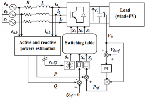
4.2 Control of the hybrid energy system grid converter using C-DPC
Figure 5. Principle of “classical DPC”
The DPC principal idea is illustrated in Figure 5. The errors amongst the momentary “active” and “reactive” powers reference values and their measurements correspond to the two “hysteresis” comparators inputs which determine, with the “switching table” help and the mains value where the mains voltage is the case of the switches. The “DC bus” voltage loop is regulated with a “PI controller” [19].
To increase precision and avert the problems confronted at the limits of each “control vector”, the “vector space” of the area is divided into twelve sectors of 30°.
4.2.1 Instantaneous power estimation
It is known that the “active” power “P” calculation is a “scalar” product between “voltages” and “currents”, whereas the “reactive” power “Q” enable to be determined by a “vector” product betwixt them [20, 21].
$P=v_a i_a+v_b i_b+v_c i_c$ (28)
$Q=\frac{1}{\sqrt{3}}\left[\left(v_b-v_c\right) i_a+\left(v_c-v_a\right) i_b+\left(v_a-v_b\right) i_c\right]$ (29)
4.2.2 Instantaneous Switching table elaboration
The “control vectors” selection is established on the variation sign produced on the “active” and “reactive” powers. Depending on the logic outputs “Sp” and “Sq” of “hysteresis comparators”, the selected vector must provide an increase or decrease in both “active” and “reactive” powers.
The same reasoning is applied for selecting the “control vectors” in the other sectors, giving the switching Table 2.
Table 2. Switching table for C-DPC
|
SP |
Sq |
θ1 |
θ2 |
θ3 |
θ4 |
θ5 |
θ6 |
θ7 |
θ8 |
θ9 |
θ10 |
θ11 |
θ12 |
|
1 |
0 |
V5 |
V6 |
V6 |
V1 |
V1 |
V2 |
V2 |
V3 |
V3 |
V4 |
V4 |
V5 |
|
1 |
V3 |
V4 |
V4 |
V5 |
V5 |
V6 |
V6 |
V1 |
V1 |
V2 |
V2 |
V3 |
|
|
0 |
0 |
V6 |
V1 |
V1 |
V2 |
V2 |
V3 |
V3 |
V4 |
V4 |
V5 |
V5 |
V6 |
|
1 |
V1 |
V2 |
V2 |
V3 |
V3 |
V4 |
V4 |
V5 |
V5 |
V6 |
V6 |
V1 |
In “F-DPC”, the conventional comparators and classical control selection table “C-DPC” are replaced by a simple “FLC”, to obtain a fixed “switching frequency”, which leads to a considerable current harmonic reduction. These rules directly use the errors of “active” and “reactive” powers as “fuzzy” variables. The control vector selection (Sa, Sb, Sc) principle is given in Figure 6 [8].
Figure 6. Principle of classical DPC
5.1 Control of the wind energy system using F-DPC
The suggested “DPC” configuration for the “wind energy system” is clarified in Figure 7.
Generally, the “FLC” design requires the choice of these parameters: “linguistic variables”, “membership functions”, “inference method”, and “fuzzification strategy”.
Figure 7. Principle control of WES based on “F-DPC”
5.1.1 Fuzzification
Fuzzy controller inputs are:
$\left\{\begin{array}{l}\varepsilon_p=P^*-P \\ \varepsilon_q=Q^*-Q\end{array}\right.$ (30)
The controller has three “membership functions” for the input of εp (“N: Negative, Z: zero, P: positive”), and two “membership functions” for the input of εq (“N: Negative, P: positive”). The memberships of the controller are illustrated in Figure 8.
5.1.2 Inference
“The fuzzy inference is the process of formulating the relationship between inputs and outputs by the fuzzy logic” [22]. These rules must take into account the system to adjust and the goals of the proposed adjustment. The “fuzzy rules” set synthesized for all “rotor flux” sectors (Table 3).
(a) active power error
(b) reactive power error
Figure 8. Membership functions
Table 3. Synthesized inference table
|
$\varepsilon_q$ |
$\varepsilon_p$ |
$\theta_1$ |
$\theta_2$ |
$\theta_3$ |
$\theta_4$ |
$\theta_5$ |
$\theta_6$ |
|
P |
N |
V3 |
V4 |
V5 |
V6 |
V1 |
V2 |
|
Z |
V7 |
V0 |
V7 |
V0 |
V7 |
V0 |
|
|
P |
V5 |
V6 |
V1 |
V2 |
V3 |
V4 |
|
|
N |
N |
V2 |
V3 |
V4 |
V5 |
V6 |
V1 |
|
Z |
V0 |
V7 |
V0 |
V7 |
V0 |
V7 |
|
|
P |
V6 |
V1 |
V2 |
V3 |
V4 |
V5 |
5.2 Control of the hybrid energy system grid converter using F-DPC
We present in this section, the DPC configuration to the “Grid Side Converter” of the “HES” using a new “Switching Table” structure. The "control vectors" selection is founded on “fuzzy rules”.
These rules directly use the “active” and “reactive” powers errors as “fuzzy variables”. The proposed DPC configuration is illustrated in Figure 9 [8].
Figure 9. Proposed structure of DPC with fuzzy selection
Table 4. Fuzzy rules
|
$\mathcal{\varepsilon}_p^{(k)}$ |
$\varepsilon_q^{(k)}$ |
$\theta_1$ |
$\theta_2$ |
$\theta_3$ |
$\theta_4$ |
$\theta_5$ |
$\theta_6$ |
$\theta_7$ |
$\theta_8$ |
$\theta_9$ |
$\theta_10$ |
$\theta_11$ |
$\theta_12$ |
|
N |
N |
V6 |
V1 |
V1 |
V2 |
V2 |
V3 |
V3 |
V4 |
V4 |
V5 |
V5 |
V6 |
|
Z |
V1 |
V1 |
V2 |
V2 |
V3 |
V3 |
V4 |
V4 |
V5 |
V5 |
V6 |
V6 |
|
|
P |
V1 |
V2 |
V2 |
V3 |
V3 |
V4 |
V4 |
V5 |
V5 |
V6 |
V6 |
V1 |
|
|
Z |
N |
V6 |
V1 |
V1 |
V2 |
V2 |
V3 |
V3 |
V4 |
V4 |
V5 |
V5 |
V6 |
|
Z |
V7 |
V0 |
V7 |
V0 |
V7 |
V0 |
V7 |
V0 |
V7 |
V0 |
V7 |
V0 |
|
|
P |
V1 |
V2 |
V2 |
V3 |
V3 |
V4 |
V4 |
V5 |
V5 |
V6 |
V6 |
V1 |
|
|
P |
N |
V5 |
V6 |
V6 |
V1 |
V1 |
V2 |
V2 |
V3 |
V3 |
V4 |
V4 |
V5 |
|
Z |
V7 |
V0 |
V7 |
V0 |
V7 |
V0 |
V7 |
V0 |
V7 |
V0 |
V7 |
V0 |
|
|
P |
V2 |
V3 |
V3 |
V4 |
V4 |
V5 |
V5 |
V6 |
V6 |
V1 |
V1 |
V2 |
At each sampling instant, the “active power” and “reactive power” errors, “εq” and “εp”, are converted into “fuzzy variables” and used to select the “control vector” allowing a better restriction of the two errors at the next sampling instant.
The “control vector” selection is by application of “fuzzy rules” (If - then) [6]. The “control vector” selection for every “fuzzy rule” is founded this time on the “sign” and the amount of variation, contrary to the “switching table” using "hysteresis comparators" logic outputs, where selection is founded solely on the “sign”.
To this effect, the digital reference values of "active" and "reactive" powers, $\varepsilon_p^{(k)}$ and $\varepsilon_q^{(k)}$, are turn into "fuzzy" variables. Three "fuzzy sets" are used to make this conversion: N, $P$ and $Z$, for each variable. The set of "fuzzy rules" combinations for all "grid voltage" sectors is shown in Table $4$.
The" HRES" utilized in this project with the “7.5 kW” DFIG and a “6 kW” "photovoltaic power system". The “HRES” model is performed in the “Matlab/Simulink” environment.
The parameters utilized in this work are given in Table 5 (appendix).
The following simulation results are divided into two parts. The first series of simulations present an evaluation of the performances of the HRES system and the second series of simulations present a comparative study between C-DPC and F-DPC.
6.1 Control evaluation of the HRES performances
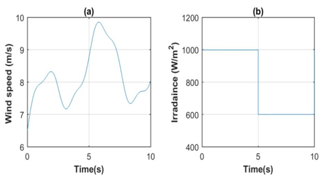
The proposed F-DPC control of HRES is tested with variable wind speed and variable solar irradiation as shown in (Figure 10). With temperature, ambient is 300 [oK].
The HRES control performances are presented in (Figure 11a), with the nominal power being 13.5 [kW]. It is observed from (Figure 11b), that the bus voltage follows the reference (620 [v]), despite considerable powers variation.
Figure 10. HRES sources
Figure 11. HRES performance
From (Figure 12), it can be noted that the grid voltage has a phase-shift of $\pi / 2$ with the HRES current; therefore, the HRES ensures a transfer of power to the grid even if the wind system operating mode (hypo-synchronous) and even variation of irradiation.
In this test, a fixed speed of 145 [rad/s] is applied to the blades of the wind turbine which corresponds to a hypo synchronous mode of the DFIG, and a constant irradiance E=1000 [w/m2].
Figure 12. Grid voltage and HRES courant
6.2 Control comparative study of C-DPC and F-DPC
The results represent a comparative study between the two direct power control techniques (classical- DPC and fuzzy-DPC).
Figure 13a shows the two active powers with “C-DPC” and “F-DPC”. It can be noted that the ripple of “active power” is considerably reduced when applying “F-DPC” as compared to the “C-DPC” technique.
According to (Figure 13b), despite the overflow at the beginning, the reactive power followed its reference with a smaller ripple when using F-DPC.
To better illustrate the impact of “F-DPC” control on the current signal quality, a spectral analysis of currents was performed. As a note, the measurement was done in the operation case of the fixed speed "wind turbine" (145 [rad/s]), but with a constant wind system "active power" (Pwind = -7 [kw]) and a unit “power factor” (Qwind = 0 [Var]), and the Photovoltaic power is (Ppv= 6 [kw]).
Figure 13. Direct power control techniques comparison
(a) classical
(b) fuzzy
Figure 14. Harmonic analysis of the HRES current spectrum
These results show that the F-DPC (Figure 14b) ensures a better quality of the HRES "current waveform", the “harmonic distortion” (THD) changes from 1.76% for the C-DPC (Figure 14a) to 1.25% for the F-DPC.
For adjusting the “switching frequency” of the converters “RSC” and “GSC” and whose purpose is to decrease the ripple power and the currents harmonics transmitted in the electrical network, the “fuzzy logic” technique has been integrated in the “DPC”.
As mentioned in the outcomes of simulation, the “F-DPC” provided a solution avoiding the “C-DPC” disadvantages.
Therefore, the common aim of this was completed in the control strategy, namely the removal of sinusoidal “currents” while reducing the “harmonic” content and ensuring unity “power factor” with a “decoupled control” of “active” and “reactive” powers.
|
DFIG |
Doubly-fed induction generator |
|
DPC |
Direct power control |
|
C-DPC |
Classical direct power control |
|
F-DPC |
Fuzzy direct power control |
|
PV |
Photovoltaic |
|
MPPT |
Maximum power point tracking |
|
DC |
Direct current |
|
S |
Circular surface swept by the turbine |
|
G |
Speed multiplier gain |
|
v |
Wind speed (m/s) |
|
ρ |
Air density |
|
λ |
Specific speed. |
|
$\sigma$ |
Dispersion coefficient |
|
$\omega_s, \omega_r$ |
Stator and rotor angular speed. |
|
Rs, Rr |
Stator resistance, rotor resistance |
|
Ls, Lr |
Inductance stator, Inductance rotor |
|
$T_r, T_s$ |
Constant stator and rotor time |
|
Msr |
Mutual inductance |
|
I |
Current generated by the cell [A] |
|
Ipv |
Photo-current generated by the cell [A] |
|
$I_d$ |
Diode current [A] |
|
$I_o$ |
Diode reverse saturation current [A]. |
|
$V$ |
Thermodynamic potential [V] |
|
$K$ |
Boltzmann's constant [ $j / k$ ]. |
|
$T$ |
Junction actual temperature [K] |
|
$q$ |
Electron charge [C]. |
|
$a$ |
P-N junction non-ideality factor ( $1 \leq a \geq 3$ ). |
Table 5. Simulation parameters.
|
Parameters |
Value |
|
DFIG |
|
|
Nominal power (P) |
7.5 [kW] |
|
Rated frequency |
50 [Hz] |
|
Stator resistance (RS) |
0.455 [Ω] |
|
Rotor resistance (RR) |
0.62 [Ω] |
|
Stator inductance (LS) |
0.084 [H] |
|
Rotor inductance (LR) |
0.081 [H] |
|
Mutual inductance (M) |
0.078 [H] |
|
Inertia (J) |
0.3125 [Kg.m2] |
|
Viscous coefficient (f) |
6.73*10-3 [N.m.s-1] |
|
Pairs of pole number (p) |
2 |
|
Wind turbine |
|
|
Nominal power |
10 [kW] |
|
Number of blades |
3 |
|
Diameter of a blade |
3 [m] |
|
Multiplier Gain |
5.4 |
|
Inertia (Jt) |
0.042 [Kg.m2] |
|
Viscous coefficient (ft) |
0.017 [N.m.s-1] |
|
PV |
|
|
Cells connected in parallel (NP) |
2 |
|
Cells connected in series (NS) |
15 |
|
Parallel resistor (RP) |
415.405 [Ω] |
|
Serie resistor (RS) |
0.221 [Ω] |
|
Junction actual temperature (T) |
25+273.15 [oK] |
|
Boltzmann's constant (K) |
1.3806503*10-23 |
[1] Zheng, J., Zhou, Z., Zhao, J., Wang, J. (2018). Integrated heat and power dispatch truly utilizing thermal inertia of district heating network for wind power integration. Applied Energy, 211(1): 865-874. https://doi.org/10.1016/j.apenergy.2017.11.080
[2] Moualdia, A., Mahmoudi, M., Nezli, L., Bouchhida, O. (2012). Modelling and control of a wind power conversion system based on the double-fed asynchronous generator. International Journal of Renewable Energy Research, 2(2): 301-306.
[3] Praveen, V., Vinay, T., Srinivasa, S. (2017). Design and implementation of direct torque controlled induction motor drive based on slip angle. International Journal of Modelling and Simulation, 37(4): 208-219. https://doi.org/10.1080/02286203.2017.1327295
[4] Djeriri, Y., Meroufel, A., Massoum, A., Boudjema, Z. (2014). A comparative study between field-oriented control strategy and direct power control strategy for DFIG. Journal of Electrical Engineering, 14(2): 169-178.
[5] Djeriri, Y. (2015). Commande directe du couple et des puissances d’une MADA associée à un système éolien par les techniques de l’intelligence artificielle., (DFIG direct torque and powers controls associated with a wind system by the artificial intelligence techniques. PhD thesis in science, Djillali liabes University, Sidi belabbas, Algeria, pp. 157-185. (In French). https://doi.org/10.13140/RG.2.1.3750.1209
[6] Belfedal, C., Gherbi, S., Sedraoui, M., Moreau, S., Champenois, G., Allaoui,T., Denaï, M. (2010). Robust control of doubly fed induction generator for stand-alone applications. Electric Power Systems Research, 80(2): 230-239. https://doi.org/10.1016/j.epsr.2009.09.002
[7] Belfedal, C., Moreau, S., Champenois, G., Allaoui, T., Denai; M. (2008). Comparison of PI and direct power control with SVM of doubly fed induction generator. Istanbul University – Journal Of Electrical & Electronics Engineering, 8(2): 633-641.
[8] Bouafia, A., Krim, F., Gaubert, J.P. (2009). Fuzzy-logic-based switching state selection for direct power control of three-phase PWM rectifier. IEEE Transactions on Industrial Electronics, 56(6): 1984-1992. https://doi.org/10.1109/TIE.2009.2014746
[9] Bouafia, A., Krim, F., Gaubert, J.P. (2009). Design and implementation of high-performance direct power control of three-phase PWM rectifier, via fuzzy and PI controller for output voltage regulation. Energy Conversion and Management, 50(1): 6-13. https://doi.org/10.1016/j.enconman.2008.09.011
[10] Elnady, A. (2018). Direct power control applied on 5-level diode clamped inverter powered by a renewable energy source. International Journal of Energy and Power Engineering, 12(6): 155-160. https://doi.org/10.5281/zenodo.1315905
[11] Tremblay, E., Atayde, S., Chandra, A. (2011). Comparative study of control strategies for the doubly fed induction generator in wind energy conversion systems: A DSP-based implementation approach. IEEE Transactions on Sustainable Energy, 2(3):288-299. https://doi.org/10.1109/TSTE.2011.2113381
[12] Piotr, P., Grzegorz, I. (2019). Direct torque control of a doubly-fed induction generator working with an unbalanced power grid. International Transactions on Electrical Energy Systems, 29(4). https://doi.org/10.1002/etep.2815
[13] Gadouche, Z., Belfedal, C., Allaoui, T., Belabbas, B. (2017). Speed-Sensorless DFIG wind turbine for power optimization using fuzzy sliding mode observer. International Journal of Renewable Energy Research, 7(2): 613-621.
[14] Assam, B., Messalti, S., Harrag, A. (2019). New improved hybrid MPPT based on backstepping-sliding mode for PV system. Journal Européen des Systèmes Automatisés, 52(3): 317-323. https://doi.org/10.18280/jesa.520313
[15] Yilmaz, U., Kircay, A., Borekci, S. (2018). PV system fuzzy logic MPPT method and PI control as a charge controller. Renewable and Sustainable Energy Reviews, 81(1): 994-1001. https://doi.org/10.1016/j.rser.2017.08.048
[16] Moutchou. R., Abbou. A. (2019) Comparative study of SMC and PI control of a permanent magnet synchronous generator decoupled by singular perturbations. 2019 7th International Renewable and Sustainable Energy Conference (IRSEC), pp. 1-7. https://doi.org/10.1109/IRSEC48032.2019.9078310
[17] Tofoli, F.L., Pereira, D.C., Paula, W.J. (2015) Comparative study of maximum power point tracking techniques for photovoltaic systems. International Journal of Photoenergy. https://doi.org/10.1155/2015/812582
[18] Benbouhenni, H., Boudjema, Z., Belaidi, A. (2019). DPC based on ANFIS super-twisting sliding mode algorithm of a doubly-fed induction generator for wind energy system. Journal Européen des Systèmes Automatisés, 53(1): 69-80. https://doi.org/10.18280/jesa.530109
[19] Shehata, E.G., Gerges, M. (2013). Direct power control of DFIGs based wind energy generation systems under distorted grid voltage conditions. International Journal of Electrical Power & Energy Systems, 53(1): 956-966. https://doi.org/10.1016/j.ijepes.2013.06.006
[20] Bouyekni, A., Taleb, R., Boudjema, Z., Kahal, H. (2018). A second-order continuous sliding mode based on DPC for wind-turbine-driven DFIG. ELEKTROTEHNIŠKI VESTNIK, 85(1-2): 29-36.
[21] Dalessandro, L., Round, S., Kolar. J. (2008). Centre-point voltage balancing of hysteresis current controlled three-level PWM rectifiers, IEEE Transactions on Power Electronics, 23(5): 2477-2488. https://doi.org/10.1109/TPEL.2008.2002060
[22] Pichan, M., Rastegar, H., Monfared, M. (2013). Two fuzzy-based direct power control strategies for doubly-fed induction generators in wind energy conversion systems. Energy, 51(2): 154-162. https://doi.org/10.1016/j.energy.2012.12.047