Ghufran W. Abedulabbas* | Farazdaq R. Yaseen
© 2022 IIETA. This article is published by IIETA and is licensed under the CC BY 4.0 license (http://creativecommons.org/licenses/by/4.0/).
OPEN ACCESS
Recently all the moving mechanical parts that are subjected to wear and cause errors in the future are replaced with the equivalent of electrical. A Brushless Direct Current (BLDC) motor is preferable compared to a brushed DC motor because it substitutes the unit of mechanical commutations with an electronic unit, enhancing dynamic properties, noise level, and efficiency. Since it is fairly inexpensive, simple in structure, and performs well, maximum BLDC motor drives use a Proportional-Integral PI controller for controlling the machine's speed. The major issue with the PI controller, on the other hand, is altering its parameters throughout the deployment. As a result, this work shows how to tune the PI controller settings of a BLDC motor drive using Grey Wolf Optimization (GWO) and Particle Swarm Optimization (PSO). The results of a comparison of PSO and GWO for BLDC motors were obtained. Simulation tests for the BLDC engine in MATLAB/Simulink environment show that both PSO and GWO of BLDC motor give good results, but the best is GWO in tested in terms of transient response under different mechanical loads and speeds.
brushless direct current (BLDC) motor, proportional-integral (PI) controller, particle swarm optimization (PSO), grey wolf optimization (GWO)
Because of their superior qualities and performance, brushless direct current motors (BLDC) have quickly acquired popularity and are now widely employed in a variety of consumer and industrial applications. A few of the advantages of BLDC motors over standard DC motors are excellent dynamic response, improved efficiency, enhanced speed versus torque properties, long-life operation, high-speed ranges, less electromagnetic interference, less noise operation, good heat dissipation, and compact size. Robotics, computer peripherals, actuation drives, machine tools, electric propulsion, and electrical power generation are all popular uses for BLDC motors [1, 2]. However, the main disadvantages are the higher cost, the size of the motor, and the requirement for a unique mounting solution for the sensors. Furthermore, Hall sensors are temperature sensitive, limiting the motor's operation, which could degrade system reliability due to the additional components and wiring [3-5]. Many researchers have used different approaches in the control speed of brushless dc motor (BLDC). In 2015, Venkata et al., [4] introduced a hybrid fuzzy PI controller for the BLDC motor speed control in electric vehicles (EV). The Hybrid Fuzzy PI controller is a combination of 2 controllers: classic PI and fuzzy PI controllers, with a selection switch which is dependent upon speed error. In the case when the speed error is over 10% of reference speed, the switch selects the FLC; or else, it selects the classic PI controller. The results reveal that the BLDC motor responds better to the Hybrid Fuzzy PI controller. Then, Yasien and Mahmood [5] presented a comparison between the new control system (NCS) and the conventional control system (CCS) of the BLDC motor. In addition, the simulation tests for BLDC motor in a MATLAB/Simulink environment show that the NCS of BLDC motor is considered better than CCS in tested in terms of transient response under different mechanical loads and speeds. After that, Aymen et al. [6] using PSO, an important metaheuristic optimization search method, this work provides a design regarding an optimal PI controller for the BLDC motor speed control.
A TMS320F28335 DSP board with MATLAB/SIMULINK interface is used in the proposed control system. Dutta and Nayak [7] through replacing a mechanical commutation unit with an electronic unit, a BLDC motor surpasses a brushed DC motor in terms of dynamic characteristics, noise reduction, and efficiency. Since it is reasonably inexpensive, simple to develop, and performs well, maximal BLDC motor drives utilize a PID controller for controlling the machine's speed. The biggest issue with PID controllers, however, is altering their parameters during deployment. Recent research has found that the Particle Swarm Optimization (PSO) approach performs well when optimizing PID controllers. The GWO algorithm is described in this work, and it is utilized for optimizing the parameters of the PID controller. The purpose of the present work is to compare the results of tuning a PID controller with the use of PSO and GWO approaches, and to conclude that the recommended strategy delivers better dynamic performance for BLDC motors. Lastly, utilizing the Artificial Bee Colony (ABC) algorithm, Vanchinatan and Selvaganesan [8] introduced adaptive Fractional Order PID (FOPID) controller for increasing the performance of BLDC motors. From previous studies, it was seen the BLDC motors demanded their high performance and reliable speed regulation under a variety of load and speed conditions.
The aim of this research is how to design a PI controller to regulate and control the speed of controlling the brushless DC motor (BLDC) and to obtain the required amplitude value for the voltage generated by the inverter, so we proposed the two famous methods of BLDC: Particle swarm optimization (PSO) and Gray Wolf Optimization (GWO) So that we know which is faster to reach an optimal value to PI Controller gains. Found that the speed error The brushless DC motor is optimized by 3% in PSO and 2% in GWO, respectively. Therefore, the results are considered satisfactory and it is proved that GWO is better than PSO.
To find the best values of Kp and Ki, two solutions have been proposed to address the response speed, the first is the PSO and GWO algorithm, both of which depend on the Integral Square Error (ISE) function as a target function to calculate the error rate, and based on it, the values of Kp and Ki were determined.
This section presents the method of the work and modelling of brushless dc motor (BLDC), Modelling is classified as:
3.1 BLDC motor’s mathematical model
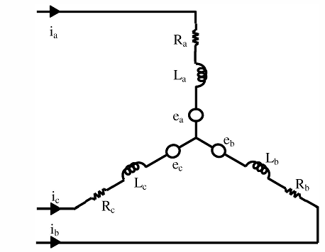
The wave-form of the applied current is rectangular, while the back electromotive force (EMF) produced by the BLDCM is trapezoidal. We'll use a 3-phase, 6-state BLDCM with Y-connected windings as well as 2-phase excitation as an example in order to make things easier. We make the next assumptions, to the extent possible: i) 3-phase windings are symmetric, ii) magnetic saturation has been ignored, iii) the hysteresis and the eddy current loss values are ignored, iv) each motor winding's inherent resistance is R, self-inductance has been represented by L, and the mutual inductance has been represented by M. Thus, the 3-phase stator voltage balancing equation could be defined using state equation below [9] Figure 1 shows the dynamic equivalent circuit of the BLDC Motor.
Figure 1. BLDC motor equivalent circuit
$\left[\begin{array}{l}V a \\ V b \\ V c\end{array}\right]=\left[\begin{array}{llr}R s & 0 & 0 \\ 0 & R s & 0 \\ 0 & 0 & R s\end{array}\right]\left[\begin{array}{l}I a \\ I b \\ I c\end{array}\right]+\left[\begin{array}{lcr}L a & L a b & L a c \\ L b a & L b & L b c \\ L c a & L c b & L c\end{array}\right] \frac{d}{d t}\left[\begin{array}{l}I a \\ I b \\ I c\end{array}\right]+\left[\begin{array}{l}e a \\ e b \\ e c\end{array}\right]$
$L a=L b=L c=L$
$L=L=L=M=0$ (1)
The induced backs EMFs have a trapezoidal form and their peak values are equal to λm w. Electromagnetic torque could be calculated through [10]:
$\begin{aligned} T e=e a I a+e b I b+e c I c / w =\lambda m(f a I a+f b I b+f c I c) \end{aligned}$ (2)
where, fa, fb, and fc have shapes like ea, eb, and e, respectively, and their maximal values are one. For a simple system with inertia Js, load torque TL, and friction coefficient Bs, the equation of motion is expressed as [9]:
$J s \frac{d w}{d t}+B s w=T e-T L$ (3)
The rotor speed (w) and the rotor position (θ), can be written as [9]:
$\frac{d \theta}{d t}=\frac{P}{2} w$ (4)
3.2 BLDC motor drive’s control system
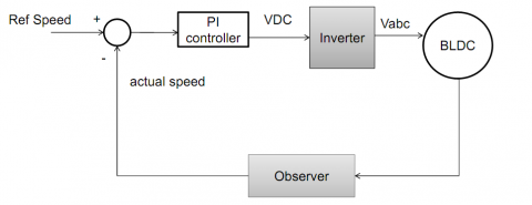
The three basic components of the BLDC motor drive control system are the BLDC motor, three-phase inverter, and control system. The block diagram design regarding the control system scheme for the BLDC motor is shown in Figure 2.
Figure 2. Diagram of a control system for BLDC motor drive
3.3 PI speed controllers
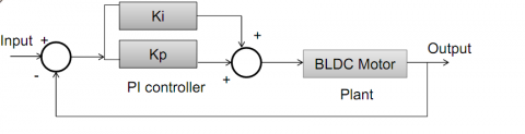
As a result of its low cost, ease of use, and capacity to be employed in various applications, the proportional-integral (PI) controller is widely used in manufacturing. It also improves the system's dynamic responsiveness and eliminates or decreases the error susceptibility and steady-state error [11]. In closed-loop control, a PI controller responds to an error signal that specifies the difference between the actual and desired signals by modifying the regulated value until the needed system response is reached [12]. Proportional integral controller (PI) contains two components of proportionate gain (Kp) and integral gain (Ki) parts. The PI controller has the general form [11]:
$u(t)=K_{p} e(t)+\int_{0}^{t} K_{i} e(t) d t$ (5)
where, u(t) represents the output of the PI controller and e(t) represents the error signal. Figure 3 shows a Proportional-Integral PI controller.
Figure 3. Block diagram representation of PI controller
4.1 Particle swarm optimization (PSO)
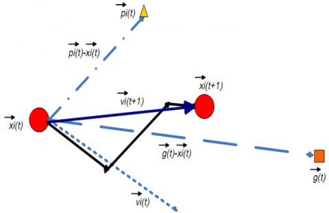
Eberhart and Kennedy first created the PSO technique in 1995 as a population-based optimization approach and a form of evolutionary computation tool. The technique was shown to be robust in addressing problems with nonlinearity and no differentiability, high dimensionality, and several optima, using adaptation, which is based on social-psychological theory. The next is the technique's properties: The approach is straightforward to implement, with great computational efficiency and a stable convergence characteristic, and it depends on swarm research, like bird flocking and fish schooling. Particles are a population of possible solutions that the PSO flow through search space. In the PSO method, particles have a variable velocity which affects how far they travel in search space. Every one of the particles has a memory as well, which allows it to recall the optimal solution in every one of the search spaces it has visited. In addition, Pbest refers to the place with the best fitness, whereas gbest refers to the overall best of the population's particles. In this work [13], PSO was utilized for tuning the weight coefficients in order to obtain an optimal controller. In PSO, a swarm of randomly selected individuals referred to as particles is produced. Each one of the particles represents a possible solution to the problem of optimization. Figure 4 shows the mathematical model is built using the following data [14].
Current Position x(t)
Current velocity v(t)
Personal Best p(t)
Global Bestg(t)
Figure 4. A mathematical model of PSO
Pseudo-code of PSO is described in Algorithm 1.
Algorithm 1 PSO
Step 1: Reading data and randomly generating an initial solution.
$x i, j=(x 1,1, x 1,2, x 1,3, \ldots \ldots \ldots \ldots xpop, n),$ i=1 to pop and j=1 to n
$v i, j=(v 1,1, v 1,2, v 1,3, \ldots \ldots \ldots \ldots vpop, n),$ i=1 to pop and j=1 to n
where, pop represents the size of the population and problem dimension.
Step 2: Calculating the objective function’s fitness value.
Step 3: Calculating the pbest, which represents the value of the objective function of every one of the particles in the current iteration’s population is compared to the preceding iteration and the particle position that has a lower objective function value as pbest for the Current iteration has been stated [15]:
pbestm ${ }^{k+1}=\left\{\right.$ pbest $m^{k}$ if $\left.f m^{k+1} \geq f m^{k}\right\}=\left\{x m^{k+1}\right.$ if $\left.f m^{k+1} \leq f m^{k}\right\}$ (6)
where, k represented the number of iterations, and f represents the objective function that has been assessed for the particle.
Step 4: Calculating the value of gbest which represents the optimal objective function that is related to pbest amongst all of the particles in that iteration is compared to that in the preceding iteration and the lower value has been chosen as the current overall gbest.
gbestm $^{k+1}=\left\{\right.$ gbestm $^{k}$ if fm$^{k+1} \geq$ fm$\left.^{k}\right\}=\left\{\right.$ pbestm $^{k+1}$ if $\left.\mathrm{fm}^{k+1} \leq \mathrm{fm}^{k}\right\}$ (7)
Step 5: Velocity update, after calculating gbest and pbest, the particles’ velocity for the following iteration must be updated with the use of equation [15]:
$v m^{k+1}=w m v m^{k}+$ C1.rand $1 \times\left(\right.$ pbesti $\left.-x m^{k}\right)+C 2$ rand $2 \times\left(\right.$ gbestm $\left.-x m^{k}\right)$ (8)
where, the above equation’s parameters have been specified in advance and ω represents the weight factor of the inertia, which has been characterized as [13]:
$w=w \max -\frac{(\text { max }-w \min )}{\text { itermax }} *$ iter (9)
C1 and C2 represent the coefficients of acceleration typically ranging within [1, 2] A large weight of the inertia (w) facilitates global search whereas the small weight facilitates the local search.
Step 6: Checking the constraints of velocity components that occur in limits from conditions below:
if vid $>$ vmax then vid $=\operatorname{vmax}($ or $)$ ifvid $<-v \max$ then vid $=-v \max$
Step 7: update the position, where every particle’s position at the following iteration (k+1) is updated as:
$x j^{k+1}=x j^{k}+v j^{k+1}$ (10)
Step 8: In the case where a number of the iterations hits the maximal value, then go to step9 for the gbest, or else, go to step 2.
Step 9: The individual generating the latest value of the gbest is optimum PI parameters at minimal objective function. The diagram for implementing the PSO algorithm has been illustrated in Figure 5.
Figure 5. The diagram for implementing the PSO algorithm
4.2 Grey wolf optimization (GWO)
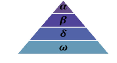
It's a metaheuristic search method inspired by grey wolf behaviour. This algorithm has been invented by (S. Mirjalili) in 2014, and its accuracy was good when compared to classic algorithms like GA, Differential calculus, PSO, and SI. The wolves in this algorithm have been placed in a pyramid shape, with levels as illustrated in Figure 6. Alpha wolves are at top of the food chain and are the group's leader, followed by the remainder of the flock. It is believed to be a helper (alpha) in decision-making at the second level, which is known as (beta). In the third level, the (Delta) sends out wolf scouts. The final level is Omega, which is for wolves who follow the dictates of the dominating wolves. Grey wolves track, chase, encircle, and attack animals as part of their hunting habit. Alpha wolves are the ones who conduct the majority of the hunting. Because these wolves have a strong understanding of prey spots, the beta may start but is directed by the alpha. As a result, three options are most appropriate for the problem. Omega wolves use alpha, beta, and delta sites to update their sites. The first ideal solution is alpha, while 2nd and 3rd ideal solutions are respectively (beta) and (delta) [7-16].
Figure 6. Hierarchy of grey wolf
In this algorithm, 4 groups have been defined, similar to the social hierarchy of the grey wolves (to live in packs), which are: Alpha (α), Beta (β), Delta (δ), and Omega (ω). Wolves’ social hierarchy has been modelled at the stage of the design. Alpha is the optimal solution, followed by β and δ as 2nd and 3rd best options. The remaining solutions are regarded as Omega since they are the least important [17].
4.2.1 Searching for prey
The grey wolves hunt for prey based on positions of the and δ. They split apart to look for the prey.
|A|>1
4.2.2 Encircling the prey
The following equations are given to quantitatively model the encircling behaviour [17]:
$\vec{D}=|\vec{C} \cdot \overrightarrow{X p}(t)-\overrightarrow{X(t)}|$ (11)
$\vec{X}(l+1)=\overrightarrow{X p}(t)-\overrightarrow{A X} \cdot \overrightarrow{D X}$ (12)
where,
$\vec{A}=2 \vec{a} \cdot \overrightarrow{r 1}-\vec{a}$ (13)
$\vec{C}=2 \cdot \overrightarrow{r 1}$ (14)
$\vec{a}=2 *\left(1-\frac{l}{l_{\max }}\right)$
t= Current iteration (15)
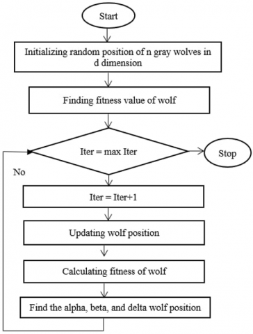
where, l is the Current iteration. $\vec{a}$ components are reduced linearly from 2 to 0 during iterations $\overrightarrow{r 1}$ & $\overrightarrow{r 2}$ represent random vectors in [0,1]. The grey wolves can encircle victims. The mathematical model assumes that the prey does not know its location. As a result, alpha, beta, and delta have more understanding concerning prey's location. The three best candidate answers are alpha (the first best solution), beta, and delta. Omega wolves reposition themselves by the upper layer wolves. In this approach, the following equations, namely themselves by the upper layer wolves. Figure 7 shows the flowchart of GWO method. In this approach, Eqns. (16), (17), and (18) are proposed [17]:
$\overrightarrow{\mathrm{D} \alpha}=|\overrightarrow{\mathrm{C} 1 \mathrm{X\cdot}} \overrightarrow{\mathrm{X} \alpha}-\overrightarrow{\mathrm{X}}|$
$\overrightarrow{\mathrm{D} \beta}=|\overrightarrow{\mathrm{C} 2 \cdot} \overrightarrow{\mathrm{X} \beta}-\overrightarrow{\mathrm{X}}|$
$\overrightarrow{\mathrm{D} \delta}=|\overrightarrow{\mathrm{C} 3 \cdot} \overrightarrow{\mathrm{X} \delta}-\overrightarrow{\mathrm{X}}|$ (16)
$\overrightarrow{\mathrm{X} 1}=\overrightarrow{\mathrm{X} \alpha}-\overrightarrow{\mathrm{A} 1} \cdot \overrightarrow{\mathrm{D} \alpha}$
$\overrightarrow{\mathrm{X} 2}=\overrightarrow{\mathrm{X} \beta}-\overrightarrow{\mathrm{A} 2} \cdot \overrightarrow{\mathrm{D} \beta}$
$\overrightarrow{\mathrm{X} 3}=\overrightarrow{\mathrm{X} \delta}-\overrightarrow{\mathrm{A} 3} \cdot \overrightarrow{\mathrm{D} \delta}$ (17)
$\overrightarrow{\mathrm{X}}(1+1)=\frac{\overrightarrow{\mathrm{X} 1}+\overrightarrow{\mathrm{X} 2}+\overrightarrow{\mathrm{X} 3}}{3}$ (18)
4.2.3 The mathematical model for hunting
The wolves advance on the prey, making the victim's position the final position of Alpha.
|A|<1
Pseudocode of GWO is described in Algorithm 2.
Algorithm 2 GOW
Initialization of grey wolf population Xi (i = 1, 2,..., n) Initialize a, A, and C
Calculating the fitness of every one of the search agents
Xα = best search agent
Xβ = 2nd-best search agent
Xδ = 3rd best search agent While (t < max number of iterations)
For every one of the search agents
Updating position of current search agent through Eq. (16)
End For
Update a, A, and C
Calculating fitness of all of the search agents Updating Xα, Xβ, and Xδ
t = t + 1 End while
Return Xα
Figure 7. Flow chart of the grey wolf optimization algorithm
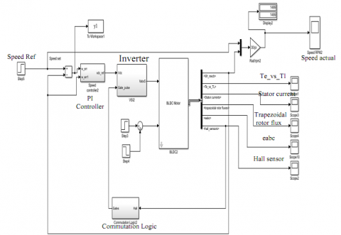
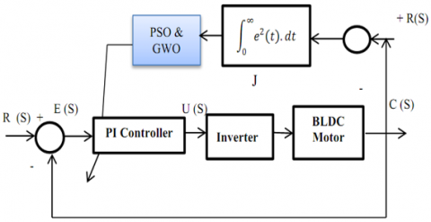
Figure 8 depicts the simulation model for PI-controlled BLDC motor drive. According to the requirements, a reference speed is set. The feedback path feeds the observed speed to the comparator. The PI controller processes the error signal. The motor's various parameters are listed in Table 1. Various algorithms are used for evaluating the PI controller's settings (KP, KI). For various systems, the GWO algorithm is used for evaluating the PI controller parameters, and the output response has been put to comparison with the PSO-based function. The PSO and GWO based PI controller design for BLDC system can be represented by the block diagram in Figure 9.
Table 1. BLDC Motor parameters
|
Rated voltage |
80 v |
|
Rated speed |
1500 rpm |
|
Rotor Inertia - J [kg-m2] Inertia, J (Kg-m2) |
5.5e-3 |
|
Resistance - Rs |
1.43ohm |
|
Inductance - Lls |
9.4e-3H |
|
Friction Coefficient -B |
2e-3 |
|
Torque constant |
10N.m |
|
Rotor Flux |
0.2158 wb |
|
Number of pole pairs (P) |
4 |
Depending on the Integrated-Square Error (ISE) between C(s) and R(s) specified as objective function J in Eq. (19), the GWO or PSO block will be fed back for minimizing the ISE to achieve appropriate PI Controller settings, i.e., Kp, Ki of PI controller producing a satisfying response.
$E(S)=R(S)-C(S)$
$J=\int_{0}^{\infty} e^{2}(t) \cdot d t$ (19)
Table 2. Basic parameter values of the algorithm
|
Algorithmic parameters |
PSO |
GWO |
|
Max. no. of search agents |
50 |
40 |
|
Iterations |
40 |
30 |
|
Dimension |
2 |
2 |
|
Lower bound |
[5 150] |
[5 150] |
|
Upper bound |
[20 500] |
[20 500] |
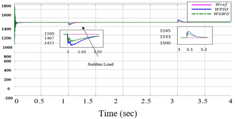
Table 2 shows the number of search agents and iterations for both methods. Comparably, Table 3 shows the KI and KP values for the two approaches. The output responses for the two cases are produced with the use of controller parameters listed in Table 4, as it has been shown in Figure 10, which shows that in the case of a GWO-based PI-controlled system, peak overshoot and settling time are shorter compared to in PSO-based system. Table 4 compares the performance of the two systems in the case when the motor is set to 1500 rpm.
Table 3. PI controller parameters for different
|
Kp |
Ki |
Speed |
algorithm |
|
9.660415791715693 |
187.2824720285225 |
1454.4 |
PSO |
|
9.9652 |
224.4844 |
1455.2 |
GWO |
|
10.7253 |
238.4021 |
1458.1 |
PSO |
|
11.8736 |
298.3538 |
1461 |
GWO |
|
12.5275 |
179.7175 |
1460 |
PSO |
|
4.229 |
193.3457 |
1463 |
GWO |
|
15.8736 |
298.3538 |
1464 |
PSO |
|
17.22086 |
246.6088 |
1467 |
GWO |
Figure 8. A BLDC Motor simulation model
Figure 9. PSO&GWO-based PI Controller design
Figure 10. Speed response in1500 rpm versus time under load 10N.m
Table 4. Performance of the PSO and GWO based PI controllers
|
Algorithm |
Rise time (s) |
Overshoot (s) |
Settling time |
|
PSO |
3.012 |
3 |
2.3 |
|
GWO |
3.015 |
2 |
2.25 |
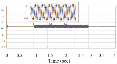
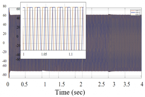
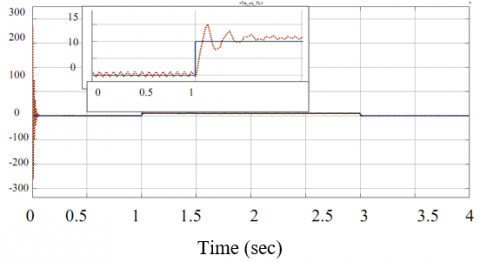
The three-phase currents for ramp response are shown in Figure 11. The magnitude current is 5 A from 0 to 0.9 sec since the motor is running at no load, and it increases to 10 while the motor is running at full load. Figure 12 show the three-phase back emf and Figure 13 Electromagnetic Torque developed in N-m.
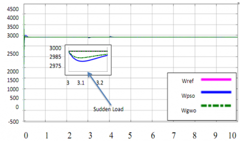
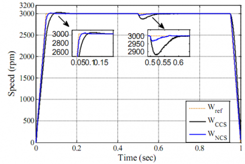
When comparing this work with another work presented in 2018 [2], which is a comparison between NCS and CCS, it was found that the results of PSO and GWO are the best from the Figure 14 and 15.
Figure 11. Three-phase stator current
Figure 12. Three Phases back emf
Figure 13. Electromagnetic Torque developed in N.m
Figure 14. Speed response in 3000 rpm versus time
Figure 15. Speed response in 3000 rpm versus time
The GWO and PSO are proposed for use in designing an optimum PI controller for the BLDC motor speed regulation in this study. Both GWO and PSO were utilized for getting the optimal reaction. A PI controller was used for controlling the BLDC speed. BDC motor's speed is controlled using a new optimization approach (GWO) which surpasses the PSO method in this research. Yet, PSO has some drawbacks, such as being easy to slip into a local optimum in a high-dimensional environment and having a slow rate of convergence. Several types of research were undertaken in the previous few decades for improving PSO. The data suggest that the machine settles down in a shorter time than the PSO-based method. Even though the GWO approach takes somewhat longer to alter the PI controller parameters regarding a BLDC motor compared to the PSO approach, the significant improvements in time domain performance justify its adoption. The suggested approach could give the field of BLDC motor drive system controller design a new dimension.
[1] Rif’an, M., Yusivar, F., Kusumoputro, B. (2018). Design of extended Kalman filter speed estimator and single neuron-fuzzy speed controller for sensorless brushless DC motor. Journal of Telecommunication, Electronic and Computer Engineering (JTEC), 10(1-5): 157-161.
[2] Akkar, H.A., Salman, S.A. (2020). Improvement parameters for design brushless DC motor by moth flame optimization. In IOP Conference Series: Materials Science and Engineering, 745(1): 012019. https://doi.org/10.1088/1757-899X/745/1/012019
[3] Sarac, V., Trajchevski, N., Golubovski, R. (2019). Assessment of the operating characteristics of brushless DC motors. Journal of Energy Technology, 12(4): 71-82. https://eprints.ugd.edu.mk/id/eprint/23891.
[4] Kommula, B.N., Kota, V.R. (2015). Performance evaluation of hybrid fuzzy pi speed controller for brushless dc motor for electric vehicle application. In 2015 Conference on Power, Control, Communication and Computational Technologies for Sustainable Growth (PCCCTSG), Kurnool, India, pp. 266-270. https://doi.org/10.1109/PCCCTSG.2015.7503912
[5] Yasien, F.R., Mahmood, R.A. (2018). Design new control system for brushless DC motor using SVPWM. International Journal of Applied Engineering.
[6] Aymen, F., Berkati, O., Lassaad, S., Srifi, M.N. (2019). BLDC control method optimized by PSO algorithm. In 2019 International Symposium on Advanced Electrical and Communication Technologies (ISAECT), Rome, Italy, pp. 1-5. https://doi.org/10.1109/ISAECT47714.2019.9069718
[7] Dutta, P., Nayak, S.K. (2021). Grey wolf optimizer based PID controller for speed control of BLDC Motor. Journal of Electrical Engineering & Technology, 16(2): 955-961. https://doi.org/10.1007/s42835-021-00660-5
[8] Vanchinathan, K., Selvaganesan, N. (2021). Adaptive fractional order PID controller tuning for brushless DC motor using artificial bee colony algorithm. Results in Control and Optimization, 4: 100032. https://doi.org/10.1016/j.rico.2021.100032
[9] Selva Pradeep, S.S., Jerisha, S. (2018). Sensorless commutation tuning based speed control of BLDC motor. Proceedings of International Conference on Energy Efficient Technologies for Sustainability, St.Xavier's Catholic College of Engineering, TamilNadu, India.
[10] Rif’an, M., Yusivar, F., Wahab, W., Kusumoputro, B. (2015). A comparison of ensemble Kalman filter and extended Kalman filter as the estimation system in sensorless BLDC motor. ARPN Journal of Engineering and Applied Sciences, 10(17): 7386-7393.
[11] Faris, F.H., Humod, A.T., Abdullah, M.N. (2019). A comparative study of pi and IP controllers for field oriented control of three phase induction motor. Iraqi Journal of Computers, Communication, Control & Systems Engineering, 19(2).
[12] Yaseen, F.R., Nasser, W.H. (2017). Design of speed controller for three-phase induction motor using the fuzzy logic approach. International Journal of Computers, Communications & Control (IJCCC), 18(3): 12. http://dx.doi.org/10.33103/uot.ijccce.18.3.2
[13] Abbas, A.I., Anwer, A. (2021). Unit commitment solution based on improved particle swarm optimization method. Engineering and Technology Journal, 39(10): 1601-1609. http://dx.doi.org/10.30684/etj.v39i10.2114
[14] Wonohadidjojo, D.M., Kothapalli, G., Hassan, M.Y. (2013). Position control of electro-hydraulic actuator system using fuzzy logic controller optimized by particle swarm optimization. International Journal of Automation and Computing, 10(3): 181-193. https://doi.org/10.1007/s11633-013-0711-3
[15] Merugumalla, M.K., Navuri, P.K. (2018). PSO and firefly algorithms based control of BLDC motor drive. In 2018 2nd International Conference on Inventive Systems and Control (ICISC), Coimbatore, India, pp. 994-999. https://doi.org/10.1109/ICISC.2018.8398951
[16] Prakash, T., Singh, V.P., Patnana, N. (2019). Gray wolf optimization-based controller design for the two-tank system. In Applications of Artificial Intelligence Techniques in Engineering, pp. 501-507. https://doi.org/10.1007/978-981-13-1819-1_47
[17] Kumar, B., Rani, A. (2018). Loss minimization in induction motor drive using grey wolf optimization. In 2018 International Conference on Computing, Power and Communication Technologies (GUCON), Greater Noida, India, pp. 770-774. https://doi.org/10.1109/GUCON.2018.8675103