Dhidik Prastiyanto* | Sutikno Madnasri | Esa Apriaskar | Nur A. Salim | Oky P. Pamungkas | Arindi Imanindi | Wahyu Caesandra | Tegoeh Tjahjowidodo
© 2022 IIETA. This article is published by IIETA and is licensed under the CC BY 4.0 license (http://creativecommons.org/licenses/by/4.0/).
OPEN ACCESS
The purpose of this work is to assess mathematical models of a digital spin coater and find the best one to represent its rotational speed behavior. Simulation models were established using a single input-output identification system approach and involved the use of multi-level periodic perturbation signals (MLPPS). The input data was taken from a Pulse-Width-Modulation (PWM) signal for the actuator in the form of MLPPS, while the observed output was from the rotational speed of the spin coater. The prospective models were represented in state-space and transfer function, both in discrete and continuous time domain. Through this study, it was found that the fitness percentage of the models obtained with the utilized approach ranged from 72% to 92% after being validated with the output of the real system. The results also indicate that for the given operating points, candidate model with discrete transfer function TFD3 has the lowest mean squared error (MSE) in average. The findings of this research may serve as a beneficial knowledge prior to controller design of the digital spin coater. Better model may lead to better controller performance that can support to perform uniformity on the film thickness.
spin coating, identification system, black-box modelling, angular velocity, MLPPS, DC motor
Thin-film deposition technology has an essential role in the development of an integrated circuit (IC). Building integration of circuits requires thin-film preparation in semiconductor production. Since demands for smaller electronic components with faster processing time are inevitable because of the industry’s automation revolution, thin-film deposition techniques have also been advancing. Several methods in a thin-film deposition have been developed, such as chemical vapor deposition (CVD) [1], physical vapor deposition (PVD) [2], and spin coating [3].
Spin coating is the most preferred method with regards to its superiorities compared to the others [4]. It is a method for depositing thin films by spreading the solution on the substrate first, and then the substrate is rotated at a constant speed to obtain evenly distributed thin film deposits on the substrate [5]. One of the advantages is the cheap manufacturing cost. It is possible to build a spin coater with a low budget and minimum power consumption but having acceptable performances [6]. Besides, the spin coating method tends to have excellent performance in terms of uniformity [7]. It is crucial to reach uniformity of thin-film production to minimize the manufactured semiconductor's error tolerances [8].
It is necessary to pay attention to the factors that affect thin films' uniformity level in terms of making a suitable spin coater. One of them is the optimal rotational disc speed [9]. The spin coater should have an excellent rotational speed control with a stable and fast response.
Several works have succeeded in getting the desired response of spinning speed through implementing the concept of a closed-loop control system. In Hossain et al. [10], the implementation utilized ATmega 32 microcontroller together with a DC motor triggered by PWM signal. The desired speed and spinning time could be set using matrix keyboard and shown through LCD display. The digital spin coater produced in that research could vary the speed up to 3000 rpm and reach the desired speed within 10 seconds. Another trial to build a digital spin coater using the closed-loop control scheme was conducted by Manikandan et al. [11]. The hardware structure was quite similar to the previous work, except for the ARM-based microcontroller used, which is well-known for its fast processing time. The system could reach the speed reference up to 3000 rpm, despite the unevaluated timing response.
However, both works did not consider involving modeling steps for designing the controller. Based on the study in Triwiyatno et al. [12], building a mathematical model of a system that can incorporates its physical dynamics encourages a more robust and better controller design [12]. It can make the spin coater become more flexible for preliminary testing of the designed controller through simulation to get the best performance.
This paper presents modeling steps for a digital spin coater. It uses the concept of a single-input and single-output identification system to generate a representative mathematical model. Since commonly a DC motor is used as the actuator of a spin coater, a PWM (Pulse Width Modulation) signal is used to drive the speed [13]. This work considers the PWM signal as an input of the spin coater system and rotational spinning speed as an output. This approach simplifies the modeling steps because it is not compulsory to get detailed information about an actuator's internal physical parameter, which can be challenging to obtain. The system's generated input applies a multi-level periodic perturbation signal (MLPPS) to produce a model with considerable fitness value.
The article is organized as follows. In section 2, the hardware and electronic design of the digital spin coater are described. The following section elaborates on how the steps conducted to model the digital spin coater. The next part aims to present results and discussions about the obtained mathematical model. Section 5 concludes the results along with suggestions for possible future research about digital spin coater.
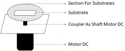
The development of a digital spin coater system considers two main steps, namely the mechanical and electronic designs. There are several parts to be noticed in the mechanical part, as shown in Figure 1(a). Figure 1(a) shows that the actuator utilized to drive the substrate is a DC motor. The 3-dimensional appearance of designed digital spin coater system can be seen in Figure 1(b). The system consists of a box with electronic components inside, where at the top part of the box, a substrate for thin film preparation, is located. As for the electronical part, the relevant components and the configuration between components must be well prepared in advance. Figure 2 illustrates the electronic design for the discussed digital spin coater system.
(a) Parts of spin coater system
(b) 3-dimensional view
Figure 1. Digital spin coater design
Figure 2. Electronic components configuration for digital spin coater
Arduino Uno microcontroller is used as the processor that connects all other components. It has considerable specifications to build a digital spin coater [6, 7]. The microcontroller uses the BTS 7960 motor driver for signal conditioning to give commands to the Brushed DC Motor. It sends pulse-width-modulation (PWM) signals to the motor driver before continuing to drive the DC motor. The encoder sensor is the component that detects the angular velocity produced by the system. Simultaneously, a Nextion LCD Touchscreen is used as an interface to adjust the rotational speed reference, spin time, and display the DC motor's real-time rotational speed value.
This study employs a system modelling method based on the concept of input and output identification of a system. In general, engineers can conduct system identification by directly applying a step signal as an input of the system, and its response in the scheme of an open-loop arrangement [14]. However, dynamic identification that involves random signals when generating input data is preferable than direct identification. The created signals enable the identification process to consider noise because its value varies with a specific frequency [15]. Dynamic identification in this study uses multi-level periodic perturbation signals as the input signals for the system.
3.1 Input-output data sets generation
The first stage in modelling of a spin coater's rotational speed is determining the input and output data sets. Several multi-level periodic perturbation signals (MLPPS) are prepared as input in the form of a PWM signal before it is used by the Arduino microcontroller to drive the DC motor, as shown in Figure 3. The motor's rotational speed detected by the rotary encoder sensor is utilized to obtain the real-time system response. Real-time system response for each input signal is managed as the corresponding output signal pair. Thus, there are four data sets, each containing input and output signal pairs, as depicted in Figure 4.
The input signal has a period Δt of 3 seconds, which is determined based on the settling time of the system defined from a given step input. With 15 times repetitions, the time spent for an input signal is 45 seconds. The PWM value that can be implemented into the spin coater system is limited from 0 to 255 because the signal used to drive a DC motor is an 8-bit PWM signal.
Figure 3. Experimental setup for input-output data sets generation
Figure 4. Input-output data set pairs of the spin coater system
3.2 Estimation of the mathematical model
Mathematical model estimation for the spin coater system was conducted using four generated data sets. Transfer function and state-space structures are utilized in this study since these structures have been considered by several studies for a system with DC motor as the actuator [16-18]. Four structures were built to express the system's model utilizing each data set; they are continuous transfer function, discrete transfer function, continuous state-space, and discrete state-space. Hence, there are sixteen candidates of models obtained from the estimation stage.
Model structures was arranged based on the differential equations of DC motor. It was started from physical equations for mechanical and electrical parts of DC motor, as listed in Eq. (1) and (2), respectively, with $\mathrm{K}$ is motor torque and electromotive force constant, $\mathrm{i}_{(\mathrm{t})}$ is armature current, b is motor viscous friction constant, $\omega_{(t)}$ is rotational speed of DC motor, $J$ is moment of inertia of the rotor, $V_{(t)}$ represents voltage source, $L$ is electric inductance, and $R$ is electric resistance.
$\mathrm{Ki}_{(\mathrm{t})}-\mathrm{b} \omega_{(\mathrm{t})}=\mathrm{J} \frac{\mathrm{d} \omega_{(\mathrm{t})}}{\mathrm{dt}}$ (1)
$\mathrm{V}_{(\mathrm{t})}-\mathrm{K} \omega_{(\mathrm{t})}=\mathrm{L} \frac{\mathrm{di}(\mathrm{t})}{\mathrm{dt}}+\mathrm{Ri}_{(\mathrm{t})}$ (2)
$\frac{\mathrm{d}}{\mathrm{dt}}\left[\begin{array}{c}\omega_{(\mathrm{t})} \\ \mathrm{i}_{(\mathrm{t})}\end{array}\right]=\left[\begin{array}{cc}\frac{-\mathrm{b}}{\mathrm{J}} & \frac{\mathrm{K}}{\mathrm{J}} \\ \frac{-\mathrm{K}}{\mathrm{L}} & \frac{-\mathrm{R}}{\mathrm{L}}\end{array}\right]\left[\begin{array}{c}\omega_{(\mathrm{t})} \\ \mathrm{i}_{(\mathrm{t})}\end{array}\right]+\left[\begin{array}{l}0 \\ \frac{1}{\mathrm{~L}}\end{array}\right] \mathrm{V}_{(\mathrm{t})}$;
$\mathrm{y}=\left[\begin{array}{ll}1 & 0\end{array}\right]\left[\begin{array}{c}\omega_{(\mathrm{t})} \\ \mathrm{i}_{(\mathrm{t})}\end{array}\right]$ (3)
From Eq. (1) and (2), we can obtain general state-space model of DC motor with $\omega_{(t)}$ as the output and $V_{(t)}$ as the input, as written in Eq. (3). Thus, it can be converted into discrete form with respect to Eq. (4), as shown in Eq. (5), with $\mathrm{T}$ represents sampling time and $\mathrm{k} \in \mathrm{Z}^{+}$. Eq. (1) and (2) can be transformed into mathematical model in the form of continuous transfer function as presented in Eq. (6). Utilizing forward rule method, Eq. (6) can be restructured into Eq. (7) that explains transfer function of DC motor in a discrete domain. Those four model structures of DC motor as shown in Eq. (3)-(7) are considered general equations for estimation process model conducted in this work.
$A=\left[\begin{array}{cc}\frac{-b}{J} & \frac{K}{J} \\ -K & -R \\ \frac{-R}{L} & \frac{-R}{L}\end{array}\right] ; B=\left[\begin{array}{l}0 \\ \frac{1}{L}\end{array}\right]$ (4)
$\left[\begin{array}{c}\omega_{((\mathrm{k}+1) \mathrm{T})} \\ \mathrm{i}_{((\mathrm{k}+1) \mathrm{T})}\end{array}\right]=\mathrm{e}^{\mathrm{AT}}\left[\begin{array}{c}\omega_{(\mathrm{kT})} \\ \mathrm{i}_{(\mathrm{kT})}\end{array}\right]+\left[\left(\mathrm{e}^{\mathrm{AT}}-\mathrm{I}\right) \mathrm{BA}^{-1}\right] \mathrm{V}_{(\mathrm{kT})}$; $\mathrm{y}=\left[\begin{array}{ll}1 & 0\end{array}\right]\left[\begin{array}{c}\omega_{(\mathrm{kT})} \\ \mathrm{i}_{(\mathrm{kT})}\end{array}\right]$ (5)
$\frac{\omega_{(s)}}{V_{(s)}}=\frac{\mathrm{K} / \mathrm{LJ}}{\mathrm{s}^{2}+(\mathrm{Lb}+\mathrm{RJ} / / \mathrm{LJ}) s+\mathrm{Rb}+\mathrm{K}^{2} / \mathrm{LJ}}$ (6)
$\frac{\omega_{(s)}}{V_{(s)}}$$=\frac{\mathrm{K} / \mathrm{LJ}}{(\mathrm{z}-1 / \mathrm{T})^{2}+(\mathrm{Lb}+\mathrm{RJ} / \mathrm{LJ})(\mathrm{z}-1 / \mathrm{T})+\mathrm{Rb}+\mathrm{K}^{2} / \mathrm{LJ}}$ (7)
3.3 Evaluation of the obtained models
Each candidate obtained from the previous step was validated with all predefined input-output pairs derived from a real-time measurement. Each validation resulted in fitness percentage that indicates the closeness of performances between obtained models and the physical system. Eq. (8) shows how the percentage value was obtained, where $\hat{p}$ is the model output signal, $p$ is the physical output, and $\bar{p}$ is its mean. The higher the fitness value, the closer the candidate model to the real system.
$\%$ fitness $=100 \times\left[1-\frac{\operatorname{norm}(p-\hat{p})}{\operatorname{norm}(p-\bar{p})} \quad \right]$ (8)
$\operatorname{MSE}=\frac{1}{\mathrm{n}} \sum_{\mathrm{i}=1}^{\mathrm{n}}(\mathrm{p}-\hat{\mathrm{p}})^{2}$ (9)
For every structure, a candidate with the best fitness percentage mean is considered as the most appropriate candidate. Thus, four best candidates from four model structures are then evaluated by comparing one to another through the value of mean squared error (MSE). Eq. (9) explains how the MSE value is obtained, with n represents the number of data for the output signal. The smaller the mean squared error, the better the candidate model resembles the system's dynamic behaviour. The chosen model is the candidate with the lowest MSE value.
The preparation of input-output pairs to find the digital spin coater system's dynamic had been conducted using Arduino Uno and produced signals depicted in Figure 4. Several model candidates were generated from those signals in continuous and discrete transfer function and state-space based on general equations as written in Eq. (3)-(7). Although the input of the system considered in this work is the integer value of the 8-bit PWM signal, it is still relevant to use those equations because PWM's value corresponds to the voltage source value. We use second-order function for obtaining all model candidates since it is suitable for modelling the angular velocity of DC motor [19]. We give each candidate different names based on its model structure and the data set used to identify the parameters. Candidates generated in a continuous transfer function structure are named with TFCx, while those in a discrete transfer function structure are named TFDx. SSCx is the name for candidates generated in continuous state-space for state-space construction, while SSDx is for discrete state-space, with x = 1, 2, 3, and 4, representing the data set utilized to build the model.
Each model candidate was evaluated by all data sets to get fitness percentages, as shown in Tables 1-4. Fitness percentage can be a suitable criterion for examining the model candidates obtained from the utilization of MLPPS in modeling a system [20]. This evaluation resulted in the best candidate for each structure. Every candidate had a different fitness percentage for every evaluation with different data sets, varying from 72% to 93%. The best fitness value was acquired by TFC3 when evaluated using data set 3 with 92.18%, while the worst ones were SSC2 and SSD2 when evaluated by data set 4, with the same value in 72.85%. However, it does not guarantee that TFC3 is the best candidate in every data set testing. When the candidates were evaluated using data set 4, the result shows that TFC4 has higher than TFC3. It also happens for SSC2 and SSD2, which are not the worst candidate when evaluated using data set 1. A model generated by a particular data set tends to have the highest fitness percentage among the other candidates when tested using the same data set. To determine the best candidate in every structure, the means of obtained fitness percentages for every candidate were calculated. TFC3, TFD3, SSC3, and SSD3 are chosen as the most promising candidates for every structure in this stage.
We can simply determine TFC3 as the best candidate for having the highest average fitness percentage in 88.55% between the chosen candidates of every structure. However, selecting the best model candidate for a spin coater should consider the rotational speed reference commonly used in spin coating application. Thin-film preparation for a dye-sensitized solar cell as one of our considered applications utilizes a spin coating method at a steady speed of 2000 rpm for 30 seconds [21]. It means that one of spin coater application uses step-response. It is appropriate to compare the model candidates' step-response model compared to the real system for the selection.
Table 1. Fitness evaluation of TFCx candidates
|
Model candidates |
% Fitness, evaluated by data set |
Mean |
||||
|
1 |
2 |
3 |
4 |
|
||
|
TFC1 |
90.68% |
86.80% |
89.25% |
77.40% |
86.03% |
|
|
TFC2 |
88.58% |
87.09% |
91.10% |
86.31% |
88.27% |
|
|
TFC3 |
89.12% |
86.62% |
92.18% |
86.29% |
88.55% |
|
|
TFC4 |
88.36% |
86.64% |
91.84% |
86.47% |
88.33% |
|
Table 2. Fitness evaluation of TFDx candidates
|
Model candidates |
% Fitness, evaluated by data set |
Mean |
||||
|
1 |
2 |
3 |
4 |
|
||
|
TFD1 |
88.60% |
86.79% |
88.71% |
73.54% |
84.41% |
|
|
TFD2 |
88.59% |
86.90% |
88.10% |
73.17% |
84.19% |
|
|
TFD3 |
86.95% |
85.57% |
90.33% |
78.67% |
85.38% |
|
|
TFD4 |
81.21% |
81.59% |
87.36% |
82.08% |
83.06% |
|
Table 3. Fitness evaluation of SSCx candidates
|
Model candidates |
% Fitness, evaluated by data set |
Mean |
||||
|
1 |
2 |
3 |
4 |
|
||
|
SSC1 |
89.73% |
88.08% |
89.54% |
73.90% |
85.31% |
|
|
SSC2 |
88.95% |
87.84% |
88.33% |
72.85% |
84.49% |
|
|
SSC3 |
87.43% |
86.23% |
91.00% |
78.65% |
85.83% |
|
|
SSC4 |
82.58% |
82.94% |
88.60% |
82.87% |
84.25% |
|
Table 4. Fitness evaluation of SSDx candidates
|
Model candidates |
% Fitness, evaluated by data set |
Mean |
|||
|
1 |
2 |
3 |
4 |
|
|
|
SSD1 |
89.73% |
88.08% |
89.54% |
73.90% |
85.31% |
|
SSD2 |
88.95% |
87.84% |
88.33% |
72.85% |
84.49% |
|
SSD3 |
87.43% |
86.23% |
91.00% |
78.65% |
85.83% |
|
SSD4 |
82.58% |
82.94% |
88.60% |
82.87% |
84.25% |
Table 5. MSE evaluation for the best in each structure
|
Model candidates |
MSE, perturbed by step-signal of PWM |
Mean |
|||
|
25% |
50% |
75% |
100% |
||
|
TFC3 |
3.7E+8 |
1.2E+9 |
1.1E+9 |
4.7E+9 |
1.8E+9 |
|
TFD3 |
3.7E+7 |
1.3E+8 |
1.3E+9 |
2.8E+9 |
1.1E+9 |
|
SSC3 |
1.1E+8 |
3.3E+8 |
2.1E+9 |
5.9E+9 |
2.1E+9 |
|
SSD3 |
1.1E+8 |
3.3E+8 |
2.1E+9 |
5.9E+9 |
2.1E+9 |
Figure 5. Step-response comparison between best model candidates and the real system when perturbed by 50% of PWM signal
$\frac{\omega(z)}{\operatorname{PWM}(\mathrm{z})}=\frac{9.009 \mathrm{z}^{-1}}{1-0.7549 \mathrm{z}^{-1}+0.04639 \mathrm{z}^{-2}}$ (10)
Figure 5 shows that TFC3 has the worst performance in resembling the real system when perturbed by a step PWM signal. For steady-state condition, TFD3, SSC3, and SSD3 have quite the same value, but when evaluated through mean squared error criterion, TFD3 has the best performance. Table 5 explains the complete evaluation of all model candidates' step-response using MSE criterion. We divide the evaluation into four operating conditions based on the system's PWM signal, representing the spin coater's speed. Since the PWM signal utilized in this work has a value between 0 to 255, PWM 50% means that it perturbs the system by 128. Based on the test, TFD3 shows the best performance for every operating condition, except for PWM 75%, which is has a higher MSE value than TFC3. However, for the average value of MSE in all operating conditions, TFD3 has the lowest value in MSE, which indicates that TFD3 is the most appropriate model among the others. Eq. (10) shows the mathematical model of TFD3.
This work contributes on the development of the mathematical model of a digital spin coater. The most appropriate model for the rotational speed of digital spin coater has been acquired. The concept of input-output identification and utilization of MLPPS were successfully employed in this work. Validation tests were conducted by evaluating the fitness percentage using given data sets and comparing the model candidates' step-response and the plant using MSE value. Model TFD3 has shown the best performance based on validation tests among all candidates. Step-response evaluation can ensure that the chosen model is the best in representing the digital spin coater's dynamics when utilized in thin-film preparation. This finding can help in simulating a designed controller for a digital spin coater using the achieved model. For future studies, investigation on artificial intelligent based model will be very interesting.
This research was carried out in the framework of the project funded by LPPM Universitas Negeri Semarang under the fundamental research grant.
[1] Pérez, E.S., Pérez, J.S., Piñón, F.M., García, J.M.J., Pérez, O.S., López, F.J. (2017). Sequential microcontroller-based control for a chemical vapor deposition process. J. Appl. Res. Technol., 15(6): 593-598. https://doi.org/10.1016/j.jart.2017.07.003
[2] Baptista, A., Silva, F.J.G., Porteiro, J., Míguez, J.L., Pinto, G., Fernandes, L. (2018). On the Physical Vapour Deposition (PVD): Evolution of magnetron sputtering processes for industrial applications. Procedia Manuf., 17: 746-757. https://doi.org/10.1016/j.promfg.2018.10.125
[3] Kelso, M.V., Mahenderkar, N.K., Chen, Q., Tubbesing, J.Z., Switzer, J.A. (2019). Spin coating epitaxial films. Science, 364(6436): 166-169. https://doi.org/10.1126/science.aaw6184
[4] Eccher, J., Zajaczkowski, W., Faria, G.C., Bock, H., von Seggern, H., Pisula, W., Bechtold, I.H. (2015). Thermal evaporation versus spin-coating: Electrical performance in columnar liquid crystal OLEDs. ACS Appl. Mater. Interfaces, 7(30): 16374-16381. https://doi.org/10.1021/acsami.5b03496
[5] Kadhim, A., Swadi, S.M., Ali, G.M. (2020). Design and implementation of a feedback programmable spin coating system. Indones. J. Electr. Eng. Comput. Sci., 17(3): 1516-1523. https://doi.org/10.11591/ijeecs.v17.i3.pp1516-1523
[6] Sadegh-cheri, M. (2019). Design, fabrication, and optical characterization of a low-cost and open-source spin coater. J. Chem. Educ., 96(6): 1268-1272. https://doi.org/10.1021/acs.jchemed.9b00013
[7] Kaddachi, Z., Belhi, M., Ben Karoui, M., Gharbi, R. (2016). Design and development of spin coating system. 17th International Conference on Sciences and Techniques of Automatic Control and Computer Engineering (STA), pp. 558-562. https://doi.org/10.1109/STA.2016.7952005
[8] Wang, B., Fu, X.H., Song, S., Chu, H., Gibson, D., Li, C., Shi, Y.J., Wu, Z.T. (2018). Simulation and optimization of film thickness uniformity in physical vapor deposition. Coatings, 8(9): 325. https://doi.org/10.3390/coatings8090325
[9] Luqman, H.H., KuZilati, K.S., Zakaria, M. (2014). Optimization of coating uniformity using modified bio-polymer in a tangential fluidized bed coater. J. Appl. Sci., 14(23): 3385-3391. https://doi.org/10.3923/jas.2014.3385.3391
[10] Hossain, M.F., Paul, S., Raihan, M.A., Khan, M.A.G. (2014). Fabrication of digitalized spin coater for deposition of thin films. International Conference on Electrical Engineering and Information & Communication Technology, pp. 1-5. https://doi.org/10.1109/ICEEICT.2014.6919158
[11] Manikandan, N., Shanthi, B., Muruganand, S. (2015). Construction of spin coating machine controlled by arm processor for physical studies of PVA. Int. J. Electron. Electr. Eng., 3(4): 318-322. https://doi.org/10.12720/ijeee.3.4.318-322
[12] Triwiyatno, A., Sumardi, S., Apriaskar, E. (2017). Robust fuzzy control design using genetic algorithm optimization approach: case study of spark ignition engine torque control. Iran. J. Fuzzy Syst., 14(3): 1-13. https://doi.org/10.22111/IJFS.2017.3238
[13] Lu, X., Chen, S., Wu, C., Li, M. (2011). The pulse width modulation and its use in induction motor speed control. 2011 Fourth International Symposium on Computational Intelligence and Design, pp. 195-198. https://doi.org/10.1109/ISCID.2011.150
[14] Sellschopp, F.S., Arjona, M.A. (2007). Semi-analytical method for determining d-axis synchronous generator parameters using the DC step voltage test. IET Electr. Power Appl., 1(3): 348-354. https://doi.org/10.1049/iet-epa:20060376
[15] Tan, A.H., Godfrey, K.R., Barker, H.A. (2015). Identification of multi-input systems using simultaneous perturbation by pseudorandom input signals. IET Control Theory Appl., 9(15): 2283-2292. https://doi.org/10.1049/iet-cta.2014.0795
[16] Abut, T. (2016). Modeling and optimal control of a DC motor. Int. J. Eng. Trends Technol., 32(3): 146-150. https://doi.org/10.14445/22315381/ijett-v32p227
[17] Elias, N., Yahya, N.M. (2018). Simulation study for controlling direct current motor position utilising fuzzy logic controller. Int. J. Automot. Mech. Eng., 154: 5989-6000. https://doi.org/10.15282/ijame.15.4.2018.19.0456
[18] Aung, Y.H., Hla, T.T. (2019). Modeling of DC motor and choosing the best gains for PID controller. Int. J. Trend Sci. Res. Dev., 3(5): 1278-1282. https://doi.org/10.31142/ijtsrd26636
[19] Amiri, M.S., Ibrahim, M.F., Ramli, R. (2020). Optimal parameter estimation for a DC motor using genetic algorithm. Int. J. Power Electron. Drive Syst., 11(2): 1047-1054. https://doi.org/10.11591/ijpeds.v11.i2.pp1047-1054
[20] Fahmizal, Arrofiq, M., Apriaskar, E., Mayub, A. (2019). Rigorous modelling steps on roll movement of balancing bicopter using multi-level periodic perturbation signals. 6th International Conference on Instrumentation, Control, and Automation (ICA), pp. 52-57. https://doi.org/10.1109/ICA.2019.8916755
[21] Madnasri, S., Wulandari, R.D.A., Hadi, S., Yulianti, I., Edi, S.S., Prastiyanto, D. (2019). Natural dye of Musa acuminata bracts as light absorbing sensitizer for dye-sensitized solar cell. Mater. Today Proc., 13: 246-251. https://doi.org/10.1016/j.matpr.2019.03.222