Mohaman Gonza* | Hassane Alla | Laurent Bitjoka
© 2022 IIETA. This article is published by IIETA and is licensed under the CC BY 4.0 license (http://creativecommons.org/licenses/by/4.0/).
OPEN ACCESS
This paper proposes an iterative control policy to design a less restrictive and admissible Petri net (PN) controller for a Discrete Event System (DES) with uncontrollable transitions, when a maximally permissive controller is not obtains by. This paper exploits a structural supervisory control method, avoiding reachability graph. This exciting method addresses the controllability condition of the desired functioning PN to define it as General Mutual Exclusion constraints (GMEC), which leads to design place invariant-based controller. The controller is non-admissible if one control place is connected to uncontrollable transition. To obtain an admissible PN controller, if such a controller exists, authors propose constraints transformation, which is computationally complex, while the controller arcs displacement approach is unsystematic. Based on it, we develop the idea to iterate the structural supervisory control method, to ensure that control place is connected to controllable transition. Through this, it was found that the displacement of arcs is systematic and the controller is less restrictive and admissible, namely the supreme controller. The results indicate that the linear constraints are never violated through the firing of uncontrollable transitions. The finding of this work may serve to evaluate the structural optimality of the controller, in order to perform it practically.
discrete event system, controllability, petri net, maximally permissive, reachability graph, supervisory control
Discrete event systems (DES) are a dynamic event-driven system with discrete state. Compared to automata, the basic tool for modeling, Petri nets (PNs) have become interesting tool for analysis and control [1, 2]. For supervisory control, synchronous product between plant and specification models helps to mitigate the state explosion and gives structurally the desired functioning PN [3]. Unfortunately, almost the supervisory control methods are based on the reachability graph, subjected again to the state explosion phenomenon [4]. Moreover, very few works have addressed the controllability condition [5], even those focused to particular PNs [6, 7].
To solve these defects, this paper exploits the structural supervisory control method [8], established to design maximally permissive controller, avoiding reachability graph and that take into account controllability condition. Indeed, from the controllability condition, defined structurally on the desired functioning PN, the Generalized Mutual Exclusion Constraints (GMEC) is expressed to design the place invariant-based controller [9]. The structure of the resulting controller is relatively simple and implemented through control places connected to plant transitions. Naturally, if the control place is connected to uncontrollable transition, the controller is non-admissible since it cannot prevent the firing of such transition. At this point, it appears necessary to find the less restrictive and admissible controller. An intuitive method is to ride up the branches of PN plant until finding a controllable transition that is upstream of the control place [10]. Unhappily, this method is not systematic and effectively applicable. Besides, some solutions based on constraints transformation or modification [11, 12] may not represent the admissible controller corresponding to the original constraint [13], while others are computationally complex. For example, the algorithm to transform a constraint into a disjunction of admissible ones proposed by Luo and Zhou [14] requires the introduction a dynamic linear constraint in order to guarantee the optimal control solution. Recently a method presented by Luo et al. [15] to design a maximally permissive controller, requires partitioning the desired functioning PN into a set of dangerous regions to deal with uncontrollable transitions. However, the control action is to maintain the greatest number of tokens not more than 1 for any sequence, contrary to the structural supervisory control where the control action is to maintain the number of tokens of specification PN more or equal to the number of tokens of the plant PN, with respect of arcs weight of transitions. In addition, there is a need for algorithm to compute the set of controllable transitions that should be disabled by the controller.
This paper establishes an iterative process based on structural supervisory control, and applies it to controlled PN, with the aim to obtain structurally the less restrictive and admissible controller. The findings shed new light on constraint transformation if one considers the complexity the concerned approaches, and the systematic control policy adapted to ride up the branches of PN plant until finding a controllable transition. The less restrictive and admissible controller is considering as the supreme controller [16].
The remainder of this paper is organized as follows: Section 2 introduces the recall on supervisory control related to controllability notion, Section 3 describes briefly the PN tool and the structural supervisory control method and in Section 4 the contribution of this paper is lights up the iterative process to structurally design supreme controller. Eventually, and in order to determine the relevance and the simplicity of the approach proposed, a case study is presented.
Supervisory control theory (SCT) of DES, based on automata, is considered as one of the most successful approaches [17]. DES are systems that evolve in accordance with the occurrence of events e and their behavior may be described as a set of sequences $\sigma$ over the alphabet $\Sigma$ (the event set). Consider the unary operator Kleene star [18], the notation $\Sigma^{*}$ gives infinite set of all possible sequences of events over $\Sigma$, including empty string $\varepsilon$.
Definition 1 (language). For a given alphabet $\Sigma$, the formal language L is a subset of $\Sigma^{*}$; it can be finite or infinite [19].
A supervisory control is a feedback control (Figure 1) where a controller C runs parallel with the plant G in order to enable/disable event occurrence based on the sequences generated by plant, so as to make the closed-loop behavior correspond to desired or legal language K. The legal behavior is defined by a given specification.
Figure 1. Basic principle of supervisory control
This principle shows that the plant coupled with controller C/G (read C controlling G) constitutes the closed-loop DES. Each time, the controller C provides a list of enabled/disabled events to occur in plant G.
The set of events $\Sigma$ may be partitioned as $\Sigma=\Sigma_{\mathrm{c}} \cup \Sigma_{\mathrm{u}}$, where $\Sigma_{\mathrm{c}}$ and $\Sigma_{\mathrm{u}}$ are, respectively, the sets of controllable events, and uncontrollable events, whose occurrence cannot be prevented by the controller. Generally, the behavior of the plant $G$ is unsatisfactory for a given specification $S$ and needs to be "restrict". Since, the desired functioning (or legal behavior) is specified by the language $K$, the basic control problem is to design a controller that restricts the closed loop behavior DES to $K \cap L(G)$. But, the presence of uncontrollable events $\Sigma_{\mathrm{u}}$, whose occurrence cannot be prevented by controller, leads to define the controllability condition.
Definition 2 (Controllability). Consider the event set $\Sigma$ of the plant $G$, partioned into the sets of uncontrollable events $\Sigma_{\mathrm{u}}$ and controllable events $\Sigma_{\mathrm{c}}$. A language $K \subseteq L(G)$ is said to be controllable with respect to the plant language $L(G)$ and $\Sigma_{\mathrm{u}}$, if
$K \Sigma_{\mathrm{u}} \cap L(G) \subseteq K$ (1)
$K \subseteq L(G)$ is prefix closed by construction; any sequence $\sigma \in K$, implies that every prefix of $\sigma$ is in $K$, i.e, $\bar{K}:=\left\{\sigma^{\prime} \in \Sigma * \mid \exists(\sigma \in K)\right.$ such $\sigma^{\prime}$ is a prefix of $\left.\sigma\right\}$.
The existence of controller $\mathrm{C}$ such that the language achieved by the closed-loop DES be $L(\mathrm{C} / \mathrm{G})=K$ is linked to the controllability condition (Eq. (1)). In the case where $K \subseteq$ $L(G)$ is not controllable with respect to the plant language $L(G)$, it is necessary to get supreme controllable language, $\operatorname{Sup} C(K)$, less permissive than $K[19]$. Thereby, the behavior of closed-loop DES is said to be maximally permissive. Regarding the automata based supervisory control, from models of given a plant $G$ and specification $S$, the Kumar's algorithm [16] allows to compute a maximally permissive controller corresponding to the supreme controllable language, such as $\operatorname{SupC}(K) \subseteq L\left(N_{S}\right) \cap L\left(N_{G}\right)$.
In this paper, we focus on structural design of such controller, avoiding the complexity linked to languages or reachability graph [5]. Thus, we will use the structural supervisory method [8], which address PN controllability condition to design the controller in the presence of uncontrollable transitions [20]. In fact, from the structure of desired functioning $\mathrm{PN}$, obtained by the synchronous product between plant PN $\left(N_{\mathrm{G}}\right)$ and specification $\mathrm{PN}\left(\mathrm{N}_{\mathrm{S}}\right)$, namely $\mathrm{N}_{\mathrm{G}} \| \mathrm{N}_{\mathrm{S}}$. The language that characterizes the trajectory of the controller satisfies [19].
$L\left(N_{G} \| N_{S}\right)=L\left(N_{S}\right) \cap L\left(N_{G}\right)$ (2)
We can get via the PN controllability condition, the linear constraints (GMEC-type) to compute the place invariantbased controller (Section 3.2), without constructing the reachability graph. The controller is admissible when control places are connected to controllable transitions of the plant $\left(N_{\mathrm{G}}\right)$. It guarantees for any $\mathrm{PN}$ state that: if transition is enabled in the plant $\left(N_{\mathrm{G}}\right)$, it must also be enabled by the specification $\left(N_{\mathrm{S}}\right)$. Nevertheless, there may exist situations where the control place is connected to uncontrollable transition, i.e, there exist uncontrollable synchronization between the controller and plant PN. Consequently, the designed controller is non-admissible, since it can never prevent plant-enabled uncontrollable transitions from firing.
In such a situation we need to obtain a less restrictive and admissible controller, such that the behavior of controlled PN (formed of the plant PN and that of the controller) being supreme controllable. For this, we propose a new idea based on the iteration of the structural supervisory control adapted to ensure there exist no arc from a control place to an uncontrollable transition by using labeled PN. This idea is explored through the classical manufacturing system where we have brought some modifications (example 1).
3.1 Petri nets tools
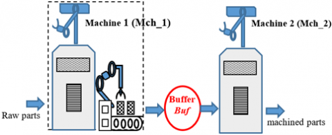
Figure 2. Topology of the modified classic manufacturing system
The power of modeling DES is strictly related to the sequences of events that it can generate. For this reason, it is suitable to use Labelled PN, which permits to specify event corresponding to transition [21]. The graphical representation of PN is given in Figure 2.
Definition 3 (Labelled PN). Let N denote a Labelled PN, it is defined to be the 7-tuplet, $N:=\left(P, T, \Sigma, D^{-}, D^{+}, M_{0}, \mathcal{L}\right)$, where
In a Labelled PN, firing a transition is linked to events occurrence, which can be portioned into uncontrollable events set $\Sigma_{u}$ and controllable events set $\Sigma_{c}$. By analogy, the set of uncontrollable transitions is denoted by $T_{u}:=$ $\left\{t_{j} \in T \mid \mathcal{L}\left(t_{j}\right) \in \Sigma_{u}\right\}$, and the controllable transitions set, $T_{c}:=$ $\left\{t_{j} \in T \mid \mathcal{L}\left(t_{j}\right) \in \Sigma_{c}\right\} .$
Example 1. Modified classic manufacturing system
The classic manufacturing system is composed of two machines (Mch_1 and Mch_2) working independently, draw raw parts upstream and reject processed parts downstream. The existing Buffer (Buf) between the machines receives the machined parts from the conveyor transfer station, after overturning. Machine (Mch_2) can only start working if it can take processed parts from the Buffer (Buf), assuming to be empty in its initial state. This modification supposes the existence of the turn over event r and transfer event v. To illustrate our contribution, we will consider that these events and the ending of the works as uncontrollable $\left(\Sigma_{\mathrm{u}}=\left\{r, v, e_{1}, e_{2}\right\}\right)$, while the starting of each machine is controllable event, $\left(\Sigma_{\mathrm{c}}=\left\{\mathrm{s}_{1}, \mathrm{~s}_{2}\right\}\right)$. We consider a given specification, which consists to ensure that a buffer $(B u f)$ has a capacity limited to $x$ parts, defined by the operator.
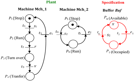
Figure 3. Labelled PN of the modified classic manufacturing system
The graphical representation of the PN of this example 1 is shown in Figure 3.
For this given example, the controllable transitions set is $T_{c}:=\left\{t_{1}, t_{4}, t_{6}\right\}$ and the uncontrollable transitions set is $T_{u}=$ $\left\{t_{2}, t_{3}, t_{5}, t_{7}\right\}$.
The PN dynamic can be represent by the presence/absence of tokens in the places. The marking or state $M$ is a column vector; $M:=P \rightarrow \mathbb{Z}$ is a mapping function that assigns a nonnegative integer (token count) to each place. For a transition $t_{j} \in T$ we define the set of input places as ${ }^{\bullet} t_{\mathrm{j}}:=\left\{p_{\mathrm{i}} \in P \mid D-\left(\bullet, t_{\mathrm{j}}\right)>0\right\}$.
If and only if $M\left(p_{\mathrm{i}}\right) \geq D-\left(\bullet, t_{\mathrm{j}}\right)$, transition $t_{\mathrm{j}}$ is enabled under $M$. From a state $M_{\mathrm{k}}$, only enabled transitions can be fired, and the new state $M_{\mathrm{k}+1}$ 'is resulted after $t_{\mathrm{j}}$ fires is denoted as $M_{\mathrm{k}}\left[t_{\mathrm{j}}\right\rangle$;
$M_{\mathrm{k}+1}=M_{\mathrm{k}}+D\left(\bullet, t_{\mathrm{j}}\right)$ (3)
where, $D\left(\bullet, t_{\mathrm{j}}\right)=D+\left(\bullet, t_{\mathrm{j}}\right)-D-\left(\bullet, t_{\mathrm{j}}\right)$ indicates for $t_{\mathrm{j}}$ the incidence matrix.
If the transition sequence $\tau \in T^{*}$ is enabled from initial state $M_{0}$, denoted as $M_{0}[\tau\rangle$ the new state is reached, denoted as $M_{0}[\tau\rangle M_{\mathrm{k}+1}$. We denote by $\mathcal{R}\left(N, M_{0}\right)$ the reachability graph, which is the set of reachable states from $M_{0}$, i.e,
$\mathcal{R}\left(N, M_{0}\right):=\left\{M_{\mathrm{k}} \in \mathbb{N} \mathrm{N} \mid \exists \tau \in T^{*} ; M_{0}[\tau\rangle\right\}$
Given a Labelled PN N, if we consider instead the transitions sequence, the events sequence (finite set) generated, then we can define PN language [21] as follows:
$L(N):=\left\{\sigma \in \Sigma^{*} \mid \exists \tau \in T^{*}, \mathcal{L}(\tau)=\sigma\right.$ and $M_{0}[\tau\rangle$ is defined $\}$
Generally, PNs can represent more expressive and prefix closed languages in $\Sigma^{*}$ than automata [22].
3.2 Structural supervisory control
The system in need of supervision, the plant and its specifications are modeled by PNs. From the desired functioning PN (Figure 4), obtained by the synchronous product between plant $\mathrm{PN}\left(N_{\mathrm{G}}\right)$ and specification $\mathrm{PN}\left(N_{\mathrm{S}}\right)$, namely $N_{\mathrm{G}} \| N_{\mathrm{S}}$, the controllability condition is established.
Figure 4. Desired functioning PN of the modified classic manufacturing system
Definition 4 (Synchronous product).
Let $N_{\mathrm{G}}:=\left(P_{\mathrm{G}}, T_{\mathrm{G}}, \Sigma_{\mathrm{G}}, D_{\mathrm{G}}^{-}, D_{\mathrm{G}}^{+}, M_{0 \mathrm{G}}, \mathcal{L}_{\mathrm{G}}\right)$ be the plant PN and $N_{\mathrm{S}}:=$$\left(P_{\mathrm{S}}, T_{\mathrm{S}}, \Sigma_{\mathrm{S}}, D_{\mathrm{S}}^{-}, D_{\mathrm{S}}^{+}, M_{0 \mathrm{~S}}, \mathcal{L}_{\mathrm{S}}\right)$ be the specification PN, both build on the same events set $\left(\Sigma_{\mathrm{S}}=\Sigma_{\mathrm{G}}\right)$. Their synchronous product $N_{\mathrm{G}} \| N_{\mathrm{S}}$ is another synchronized Petri net, $N:=\left(P, T, \Sigma, D^{-}, D+, M_{0}, \mathcal{L}\right)$, such that
Intuitively, the synchronous product is a matter of structural synchronization, where a pair of transitions $\left(t_{\mathrm{G}}, t_{\mathrm{S}}\right)$ with the same event is replace with a single transition $t_{\mathrm{j}}=\left(t_{\mathrm{G}}, t_{\mathrm{S}}\right)$, Particularly, called synchronous transition. If there exist several transitions in each PN with the same event, then there exists one transition in the desired functioning PN for each transition pair combination (Kumar and Holloway, 1996). Without loss this generality, we applying this suitable operation to the PN of Figure 3, where each event is associated with at most one transition in each PN.
From a desired functioning PN we can check the controllability condition, because the structural synchronization via uncontrollable transitions can be a potential source of uncontrollability and forbidden states [23, 24].
Definition 5 (Forbidden states). Let $t_{j}=\left(t_{G}, t_{S}\right) \in T_{u}$ be a synchronous transition in desired functioning $\mathrm{PN}, M_{G}\left(\bullet_{j}\right)$ and $M_{S}\left({ }^{\bullet} t_{j}\right)$ the marking of input places belongs to plant $N_{P}$ and specification $N_{S}$ respectively; we define the set of forbidden states.
$\mathcal{M}_{b}:$$=\left\{M_{k} \in \Re\left(N, M_{0}\right) \mid \exists t_{j}=\left(t_{G}, t_{S}\right) \in T_{u}\right.$, such that $\left\{\begin{array}{l}M_{G}\left({ }^{\bullet} t_{j}\right) \geq D_{G}^{-}\left(\bullet t_{j}\right) \\ M_{S}\left(\bullet t_{j}\right)<D_{S}^{-}\left(\bullet t_{j}\right)\end{array}\right\}$
The desired functioning $\mathrm{PN}, N:=N_{G} \| N_{S}$, is uncontrollable when a reachable state $M_{k} \in \mathcal{M}_{b}$. In the Figure 4 we face such situation when we consider the uncontrollable synchronous transition $t_{4}$, namely,
$t_{4} \in T_{u} ;\left\{\begin{array}{c}M_{G}\left(P_{4}\right) \geq 1 \\ M_{S}\left(P_{8}\right)<M_{G}\left(P_{4}\right)\end{array}\right.$
This allows defining structural controllability condition of the desired functioning PN.
Definition 6 (structural controllability). For any uncontrollable synchronous transition $t_{j}=\left(t_{G}, t_{S}\right) \in T_{u}$, the structural controllability condition for any reachable state $M_{k}$, when $M_{P}\left({ }^{\bullet} t_{j}\right) \geq D_{G}^{-}\left(\bullet t_{j}\right)$ is [8].
$M_{S}\left({ }^{\bullet} t_{j}\right) \geq M_{G}\left({ }^{\bullet} t_{j}\right)$, wiht $M_{S}\left({ }^{\bullet} t_{j}\right) \geq D_{S}^{-}\left(\bullet t_{j}\right)$ (4)
It has been proven that the structural controllability condition is equivalent to that defined on the PN languages.
$M_{S}\left({ }^{\bullet} t_{j}\right) \geq M_{G}\left({ }^{\bullet} t_{j}\right) \Leftrightarrow K \Sigma_{u} \cap L\left(N_{G}\right) \subseteq K$
From this it is seem not necessary scanning the reachability graph or PN languages to check the controllability and to define a set of admissible states.
Definition 7 (Admissible states). Given a desired functioning PN, the set of admissible states, $\mathcal{M}_{\mathrm{a}}$, is the one in which the structural controllability condition is verified.
$\mathcal{M}_{\mathrm{a}}:=\left\{M_{k} \in \mathfrak{R}\left(N, M_{0}\right) \mid \exists t_{j}=\left(t_{G}, t_{S}\right) \in T_{u} ; M_{S}\left(\cdot t_{j}\right) \geq M_{G}\left(\bullet_{j}\right)\right\}$
The controllability condition can be is expressed into linear constraints of GMEC type, denoted as $L^{T} M_{k} \leq b, \forall M_{k} \in \Re\left(N, M_{0}\right)$, where, $L=\left[l_{1} \cdots l_{n}\right] \in \mathbb{Z} n_{c} \times m$ and $b \in \mathbb{Z}^{n_{c}}$.
For any $t_{j}=\left(t_{G}, t_{S}\right) \in T_{u}$ the controllability condition is expresses into inequality $M_{G}\left(\cdot t_{j}\right)-M_{S}\left(\cdot t_{j}\right) \leq 0$, where, $L=$ $\left[0 \cdots 0 l_{G} 0 \cdots 0 l_{S} 0 \cdots 0\right]$, with $l_{G}=1, l_{S}=-1$ and $b=0$.
Hence, in the Figure 4 , the controllability condition is $M_{S}\left(P_{8}\right) \geq M_{G}\left(P_{4}\right)$ and the corresponding constraint is $L=$$\left[\begin{array}{lllllll}0 & 0 & 0 & 1 & 0 & 0 & 0-1\end{array}\right]$.
At this point, the control goal is to ensure that the constraints are met during the plant's operation. At this point, the place invariant method provides the controller incidence matrix $D_{C}$ and initial state $\mathrm{M}_{0 \mathrm{C}}$ of the $\mathrm{PN}$ that implements a controller $C[22]$. The place invariant based controller identical to the monitors $[7,20]$. The controller is a $P N$ with incidence matrix $D_{C} \in \mathbb{Z}^{n_{C} \times m}$ with initial state $M_{0 C} \in \mathbb{Z}^{n_{c}}$, made up of the plant's transitions and a separate set of places.
$D_{C}=-L D, M_{0 C}=-L M_{0}$ (5)
The controller is maximally permissive assuming that the plant's transitions are controllable.
Definition 8 (maximally permissive controller). A controller is maximally permissive if all the admissible state, $\mathcal{M}_{\mathrm{a}}$ of the desired functioning $\mathrm{PN}, N:=N_{G} \| N_{S}$, are reachable under control, and the firing of transitions that leads the plant $\mathrm{PN}$ evolution to a forbidden state is prevented.
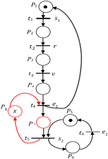
In incidence matrix $D_{C}$ positive elements in refer to arcs connecting transitions to control places and negative elements refer to arcs connecting control places to transitions. From this, the controller C is coupled by synchronization to desired functioning PN, to give the controlled PN (Figure 5).
Figure 5. The controlled PN of the modified classic manufacturing system
Definition 9 (Controlled PN). A controlled PN is a triple $\mathcal{N}=$ $(N, C, B)$; where $N:=N_{G} \| N_{S}$ is the desired functioning $\mathrm{PN}, C$ a PN model of the controller is a finite set of control places, $C \cap P=$ $\emptyset$, and $B \subseteq C \times T$ is a set of arcs (with weight) connecting control places $\left(p_{c}\right)$ to transitions set $T$.
Applying this to our current example 1 (Figure 4), we have:
$D_{C}=-\left[\begin{array}{lllllll}0 & 0 & 0 & 1 & 0 & 0 & 0-1\end{array}\right]\left[\begin{array}{cccccc}-1 & 0 & 0 & 1 & 0 & 0 \\ 1 & -1 & 0 & 0 & 0 & 0 \\ 0 & 1 & -1 & 0 & 0 & 0 \\ 0 & 0 & 1 & -1 & 0 & 0 \\ 0 & 0 & 0 & 0 & -1 & 1 \\ 0 & 0 & 0 & 0 & 1 & -1 \\ 0 & 0 & 0 & 1 & -1 & 0 \\ 0 & 0 & 0 & -1 & 1 & 0\end{array}\right]$$=\left[\begin{array}{llllll}0 & 0 & -1 & 0 & 1 & 0\end{array}\right]$
$M_{0 C}=-\left[\begin{array}{lllllll}0 & 0 & 0 & 1 & 0 & 0 & 0-1\end{array}\right]\left[\begin{array}{l}1 \\ 0 \\ 0 \\ 0 \\ 1 \\ 0 \\ 0 \\ x\end{array}\right]=x$
In controlled PN, the controller must allow all control (connected) transitions to be fired only when it is both control place and plant enabled, otherwise it is prevented. Consider the control transition $t_{3} \mid \mathcal{L}\left(t_{3}\right)=v$ as controllable, then the controller designed is maximally permissive. Unfortunately, it was specified (section 2) that the event $v$ is uncontrollable, i.e, the transition $t_{3} \mid \mathcal{L}\left(t_{3}\right)=v$ is uncontrollable. Hence, the controller designed is non-admissible, since it cannot prevent such transition when it is enabled in plant PN. The controllability of the controlled PN must be checked, in order to obtain the less restrictive and admissible controller (supreme controller). In fact, the controller designed may prevent plant-enabled uncontrollable transitions from firing.
Uncontrollable transitions can cause problem for controlled PN, due to arcs from the control places used to change the controller state based on the firings of plant transitions. For this reason, we propose an idea for structurally design the supreme controller, which is less restrictive and admissible. For each control (connected) transition $t_{\mathrm{j}} \in T$ of the controlled $\mathrm{PN}, \mathcal{N}=(N, C, B)$, where $M_{N}\left({ }^{\cdot} t_{j}\right)$ is the marking of input places belonging to plant $N_{\mathrm{G}}$, and $M_{C}\left({ }^{\cdot} t_{j}\right)$ is the marking of input control places belonging to controller $C$. When the controller behaves correctly the connected transition $t_{j}$ must be disabled if the marking of input control places $M_{C}\left({ }^{\cdot} t_{j}\right)$ is less than weigh of their $\operatorname{arcs} B\left(\bullet t_{j}\right)$, i.e, $M_{C}\left({ }^{\cdot} t_{j}\right) \geq B\left(\bullet t_{\mathrm{j}}\right)$. When the connected transition is uncontrollable $\left(t_{\mathrm{j}} \in T_{\mathrm{u}}\right)$, there is no guarantee that will happen, since the firing of such transition is limited solely by the structure and state of the plant $N_{\mathrm{G}}$. Consequently, the controller designed is non-admissible [11]. Given $\mathrm{D}$ the incidence matrix of $N:=N_{\mathrm{G}} \| N_{\mathrm{S}}$ and $\mathrm{L}=\left[0 \cdots 0 l_{\mathrm{G}} 0 \cdots 0 l_{\mathrm{S}} 0 \cdots 0\right]$ the constraint from controllability condition $M_{\mathrm{S}}\left({ }^{\cdot} t_{\mathrm{j}}\right) \geq M_{\mathrm{G}}\left({ }^{\cdot} t_{\mathrm{j}}\right)$. Let $D_{\mathrm{u}}$ be sub-matrix representing the uncontrollable part of $D$, such that $L D_{\mathrm{u}}$ is the portion of controller corresponds to uncontrollable transitions. Let's see $L D_{\mathrm{u}}$ like the admissibility condition of designed controller. If $L D_{\mathrm{u}}$ contains at least one strictly positive element, i.e $L D_{\mathrm{u}} \geq 0$, then there is control place connected to uncontrollable transition $\left(t_{\mathrm{j}} \in T_{\mathrm{u}}\right)$.
Consider in our example (Figure 4) the uncontrollable transitions set $T_{u}=\left\{t_{2}, t_{3}, t_{4}, t_{6}\right\}$ associated by label function to the uncontrollable events set transitions $\Sigma_{u}=\left\{r, v, e_{1}, e_{2}\right\}$ we will have,
$L D_{u}=\left[\begin{array}{llllllll}0 & 0 & 0 & 1 & 0 & 0 & 0 & -1\end{array}\right]\left[\begin{array}{cccc}0 & 0 & 1 & 0 \\ -1 & 0 & 0 & 0 \\ 1 & -1 & 0 & 0 \\ 0 & 1 & -1 & 0 \\ 0 & 0 & 0 & 1 \\ 0 & 0 & 0 & -1 \\ 0 & 0 & 1 & 0 \\ 0 & 0 & -1 & 0\end{array}\right]$$=\left[\begin{array}{llll}0 & 1 & 0 & 0\end{array}\right]$
For the controller to be less restrictive and admissible, the sufficient condition should be $L D_{u} \leq 0$, where the constraint $L=$ $\left[0 \cdots 0 l_{G} 0 \cdots 0 l_{S} 0 \cdots 0\right]$ is given by controllability condition $M_{S}\left({ }^{\cdot} t_{j}\right) \geq M_{G}\left({ }^{\cdot} t_{j}\right)$.
When the condition $L D_{u} \leq 0$ is unsatisfied, the idea is to iterate the structural supervisory control method from the controlled PN until founding controllable transitions, which is upstream to the control places. Concretely, it is a question of extending the controllability condition to the controlled $\mathrm{PN}, \mathcal{N}=(N, C, B)$. Hence, for any uncontrollable control transition $t_{j} \in T_{u}$, the structural controllability condition for any reachable state $M_{k}$, when $M_{N}\left({ }^{\bullet} t_{j}\right) \geq D-\left(\bullet t_{j}\right)$ is
$M_{C}\left({ }^{\cdot} t_{j}\right) \geq M_{N}\left({ }^{\cdot} t_{j}\right)$ with $M_{C}\left({ }^{\cdot} t_{j}\right) \geq B\left(\bullet t_{j}\right)$ (6)
Corollary. Let $L_{\mathcal{N}}=\left[0 \cdots 0 l_{N} 0 \cdots 0 l_{C} 0 \cdots 0\right]$ be a constraint provided by an extending controllability condition $M_{C}\left({ }^{\cdot} t_{j}\right) \geq M_{N}\left({ }^{\cdot} t_{j}\right)$ to the controlled $\mathrm{PN}, \mathcal{N}=(N, C, B)$, and $D_{\mathcal{N} u}$ be the incidence sub-matrix representing the uncontrollable part of $D_{\mathcal{N}}$ The new controller $C_{1}$ is admissible, while the condition $L_{\mathcal{N}} D_{\mathcal{N} u} \leq 0$.
Proof. If the control place is connected to uncontrollable trans1tion, the (extended) controllability condition $M_{C}\left({ }^{\bullet} t_{j}\right) \geq M_{N}\left({ }^{\bullet} t_{j}\right)$ is satisfied. The constraint $L$ is systematically transformed to a new one, $L_{\mathcal{N}}$ in order to enforce the condition $L_{\mathcal{N}} D_{\mathcal{N} u} \leq 0$. By iteration of the structural controller design, this will result to connecting control place to a controllable transition, since the number of plant transitions is finite.
Consider the desired functioning $\mathrm{PN}, N:=N_{\mathrm{G}} \| N_{\mathrm{S}}$ with controllability condition $M_{S}\left({ }^{\bullet} t_{j}\right) \geq M_{G}\left({ }^{\bullet} t_{j}\right)$ and the admissibility condition of controller $L D_{\mathrm{u}} \geq 0$, one can then find a less restrictive and admissible controller using Algorithm 1.
Algorithm 1: Structural design of a supreme controller (less restrictive and admissible.
Input: controlled PN, $\mathcal{N}=(N, C, B)$ and $D_{\mathcal{N}}$
Output: supreme controller $C_{i}$,
Initialization step: From controlled $\mathrm{PN}, \mathcal{N}=(N, C, B)$ check if the controller $C$ draws no arc to uncontrollable transition $\left(t_{j} \in T_{u}\right)$, i.e., $L D_{u} \leq 0$.
1: If not, set $L_{\mathcal{N}}=\left[0 \cdots 0 l_{N} 0 \cdots 0 l_{C} 0 \cdots 0\right]$ is constraint provided by $M_{C}\left({ }^{\bullet} t_{j}\right) \geq M_{N}\left({ }^{\bullet} t_{j}\right)$.
Supreme control step:
2: Do i:=1, $D_{C_{1}}=-L_{\mathcal{N}} D_{\mathcal{N}}$ and check $L_{\mathcal{N}} D_{\mathcal{N} u}$, where $D_{\mathcal{N} u}$ is the sub-matrix representing the uncontrollable part of $D_{\mathcal{N}}$
3: If $L_{\mathcal{N}} D_{\mathcal{N} u} \leq 0, C_{1}$ is less restrictive and admissible controller
4: If not i.e $L_{\mathcal{N}} D_{\mathcal{N} u} \neq 0$,
5: Repeat (1) for the next controller PN $\mathcal{N}_{1}=\left(N, C_{1}, B_{1}\right)$
6: Do $D_{C_{i}}=-L_{\mathcal{N}_{i-1}} D_{\mathcal{N}_{i}-1}$ and check $L_{\mathcal{N}_{i-1}} D_{\mathcal{N}_{i-1} u}$
i: =i+1,
7: Until $L_{\mathcal{N}_{i-1}} D_{\mathcal{N}_{i-1}} \leq 0$
Stop. $C_{i}$ is less restrictive and admissible controller
8: For all $\left(t_{j} \in T\right)$ if we have always $L_{\mathcal{N}_{i-1}} D_{\mathcal{N}_{i-1} \quad u} \nleq 0$, then the control solution is empty, $\left(C_{i}=\emptyset\right)$. This is good solution, since the plant PN transitions is finite.
Let us apply the above to controlled PN (Figure 5) of our current example 1 where the controller is non-admissible, because it is connected to the uncontrollable transition, $t_{3} \mid \mathcal{L}\left(t_{3}\right)=v$.
Iteration or step 1
The characteristics of the controlled PN are
$D_{\mathcal{N}}=\left[\begin{array}{cccccc}-1 & 0 & 0 & 1 & 0 & 0 \\ 1 & -1 & 0 & 0 & 0 & 0 \\ 0 & 1 & -1 & 0 & 0 & 0 \\ 0 & 0 & 1 & -1 & 0 & 0 \\ 0 & 0 & 0 & 0 & -1 & 1 \\ 0 & 0 & 0 & 0 & 1 & -1 \\ 0 & 0 & 0 & 1 & -1 & 0 \\ 0 & 0 & 0 & -1 & 1 & 0 \\ 0 & 0 & -1 & 0 & 1 & 0\end{array}\right]$ and $M_{0_{\mathcal{N}}}=\left[\begin{array}{l}1 \\ 0 \\ 0 \\ 0 \\ 1 \\ 0 \\ 0 \\ x \\ x\end{array}\right]$
We put in red the columns corresponds to $D_{\mathcal{N u}}$;
The controllability condition is $M_{C}\left(P_{c}\right) \geq M_{P}\left(P_{3}\right)$;
The constraint is $L_{\mathcal{N}}=\left[\begin{array}{llllllll}0 & 0 & 1 & 0 & 0 & 0 & 0 & 0\end{array}\right.$;
The new controller is $\left\{\begin{array}{c}D_{C_{1}}=\left[\begin{array}{cccccc}0 & -1 & 0 & 0 & 1 & 0\end{array}\right] \text {; } \\ M_{0 C_{1}}=x\end{array}\right.$
The controller portion corresponding to uncontrollable transitions $L_{\mathcal{N}} D_{\mathcal{N} u}=\left[\begin{array}{llll}1 & 0 & 0 & -1\end{array}\right]$.
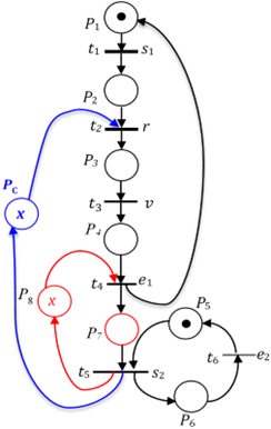
The resulting controller is non-admissible, since $L_{\mathcal{N}} D_{\mathcal{N} u} \nleq 0$ one strictly positive element) and $D_{C_{1}}$ draws an arc to the supposed uncontrollable transition $t_{2} \mid \mathcal{L}\left(t_{2}\right)=r$ (Figure 6). Consequently, we must iterate the procedure again.
Figure 6. Controlled $\mathrm{PN} \mathcal{N}_{1}$, after $1^{\text {st }}$ step, with non-admissible controller $C_{1}$
Iteration or step 2
Characteristic of controlled PN
$D_{\mathcal{N}_{1}}=\left[\begin{array}{cccccc}-1 & 0 & 0 & 1 & 0 & 0 \\ 1 & -1 & 0 & 0 & 0 & 0 \\ 0 & 1 & -1 & 0 & 0 & 0 \\ 0 & 0 & 1 & -1 & 0 & 0 \\ 0 & 0 & 0 & 0 & -1 & 1 \\ 0 & 0 & 0 & 0 & 1 & -1 \\ 0 & 0 & 0 & 1 & -1 & 0 \\ 0 & 0 & 0 & -1 & 1 & 0 \\ 0 & -1 & 0 & 0 & 1 & 0\end{array}\right]$ and $M_{0 \mathcal{N}_{1}}=\left[\begin{array}{l}1 \\ 0 \\ 0 \\ 0 \\ 1 \\ 0 \\ 0 \\ x \\ x\end{array}\right]$
The controllability condition is $M_{C}\left(P_{c}\right) \geq M_{P}\left(P_{2}\right)$.
The constraint is $L_{\mathcal{N}_{1}}=\left[\begin{array}{llllllll}0 & 1 & 0 & 0 & 0 & 0 & 0 & 0-1\end{array}\right]$.
The new controller is $\left\{\begin{array}{c}D_{C_{2}}=\left[\begin{array}{cccccc}-1 & 0 & 0 & 0 & 1 & 0\end{array}\right] \\ M_{0 C_{2}}=x\end{array}\right.$.
The controller portion corresponding to uncontrollable transitions $L_{\mathcal{N}_{1}} D_{\mathcal{N}_{1} u}=\left[\begin{array}{llll}0 & 0 & 0 & -1\end{array}\right]$.
This solution is less restrictive and admissible because $L_{\mathcal{N}_{1}} D_{\mathcal{N}_{1} u} \leq 0$ (none strictly positive element) and $D_{C}$ will draw an arc to the controllable transition $t_{1} \mid \mathcal{L}\left(t_{1}\right)=s_{1}$ (Figure 6). We must stop the iteration here, because we get the supreme controller.
The approach is systematic and structural, since we find the solution similar to the intuitive approach of Yamalidou et al. [10]. Now, suppose that transition $t_{1} \mid \mathcal{L}\left(t_{1}\right)=s_{1}$ is uncontrollable transition, then the control solution is empty. It can be noticed that, in Figure 6 place P8 is implicit and can be suppressed.
Remark 1. Modeling considerations
Example 1 shows typical modeling plant PN’s structures. It can be seen that the uncontrollable transition has only one input place. This is in fact a general modeling aspect, which leads us to precise the modeling characteristics of controllable and uncontrollable transitions.
Controllable transition: A controllable transition may have several input places. Indeed, the firing of this transition is conditioned by the synchronization of several tasks behaving concurrently. The controllable transition is fired when all the input places are marked and the controllable event occurs.
Uncontrollable transition: An uncontrollable transition has only on input place. The occurrence of an uncontrollable event, a breakdown or the end of a task for example cannot be blocked by several input places. It occurs when the plant is in a given state, represented in a global way by the input place.
Compare to existing methods (constraint transformation or algorithm to compute controllable transitions), we have presented a very simple idea, systematic and easy to implement by using the iteration of structural supervisory control with respect of controllability condition. Also, the simplicity of linear constraints allows obtaining a controller structurally optimal (no addition of control places or arcs to the controlled PN). This solution problem has already been tackled by Yamalidou et al. [10] in an intuitive and unsystematic way. We assume that, a good variety of DES control problems can be efficiently solved through advantages of this approach:
As a case study, consider the real-life system taken from Ref. [25]. It is in an industrial assembly line, whose topology is illustrated in Figure 7.
Figure 7. Controlled PN $\mathcal{N}_{2}$, after 2 nd step, with supreme controller $C_{2}$
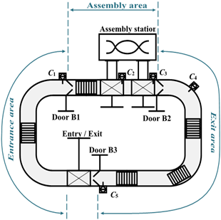
Figure 8. Topology of industrial assembly line [10]
The assembly line consists of a conveyor, an assembly station, three barrier doors (B1-3) and five sensors (C1-5). An entry / exit station connects the assembly system with other systems in the line and provides entry / exit of parts into the assembly loop. The assembly loop is divided into three areas:
A part enters the system through the entry / exit station, travels the entry area, and then is admitted into the assembly area, where it is introduced inside the assembly station to be processed. Once it is complete, the assembled parts are returned to the conveyor, travel through the exit area and exit the assembly loop via the entry / exit station. The system (assembly line) must satisfy the following specifications:
The PNs of Figure 8, models the plant and the specification of the assembly line, while events associated with transitions and the place descriptions are shown in Table 1.
Table 1. Description of places and events associated with transitions
|
Places |
|
|
P1 |
There is no room at the entrance to the assembly area |
|
P2 |
Part waiting to enter the assembly area |
|
P3 |
Part entering the assembly area |
|
P4 |
Part entered in the assembly area |
|
P5 |
No part is awaiting assembly |
|
P6 |
Part awaiting assembly |
|
P7 |
Part being assembled |
|
P8 |
Part waiting to leave the assembly area |
|
P9 |
Part leaving the assembly area |
|
P10 |
Part taken out of the assembly area |
|
P11 |
There are no parts waiting to leave the assembly loop |
|
P12 |
Piece waiting to leave the assembly loop |
|
P13 |
Piece leaving the assembly loop |
|
P14 |
Piece taken out of the assembly loop |
|
P15 |
Current number of parts in the assembly area |
|
P16 |
Number of parts waiting to leave the assembly loop |
|
P17 |
Number of places available in the assembly queue |
|
P18 |
Number of places occupied in the assembly queue |
|
P19 |
Number of places available in the exit queue |
|
P20 |
Number of places occupied in the exit queue |
|
Transitions |
|
|
c1a |
There is no room at the entrance to the assembly area |
|
b1o |
Part waiting to enter the assembly area |
|
c1i |
Part entering the assembly area |
|
b1f |
Part entered in the assembly area |
|
c2a |
No part is awaiting assembly |
|
Da |
Part awaiting assembly |
|
c3a |
Part being assembled |
|
b2o |
Part waiting to leave the assembly area |
|
c4a |
Part leaving the assembly area |
|
b2f |
Part taken out of the assembly area |
|
c5a |
There are no parts waiting to leave the assembly loop |
|
b3o |
Piece waiting to leave the assembly loop |
|
c5i |
Piece leaving the assembly loop |
|
b3f |
Piece taken out of the assembly loop |
All forbidden states $\mathcal{M}_{b}$ are consequences of the synchronization of plant $\mathrm{PN}$ with specification $\mathrm{PN}$ via uncontrollable transitions: $t_{4}\left|\mathcal{L}\left(t_{4}\right)=b 1 f, t_{10}\right| \mathcal{L}\left(t_{10}\right)=b 2 f$ and $t_{14} \mid \mathcal{L}\left(t_{14}\right)=b 3 f$. To ensure the respect of the specification, it is therefore necessary to define the controllability condition, namely
$\left\{\begin{array}{l}M_{S}\left(P_{17}\right) \geq M_{P}\left(P_{4}\right) \\ M_{S}\left(P_{18}\right) \geq M_{P}\left(P_{10}\right) \\ M_{S}\left(P_{19}\right) \geq M_{P}\left(P_{10}\right) \\ M_{S}\left(P_{20}\right) \geq M_{P}\left(P_{14}\right)\end{array}\right.$
The constraint L is in following equation.
The characteristic of desired functioning PN (Figure 9).
The controller of the assembly line can therefore be computed, that is in following equation (DC).
$L=\left[\begin{array}{llllllllllllllllllll}0 & 0 & 0 & 1 & 0 & 0 & 0 & 0 & 0 & 0 & 0 & 0 & 0 & 0 & 0 & 0 & -1 & 0 & 0 & 0 \\ 0 & 0 & 0 & 0 & 0 & 0 & 0 & 0 & 0 & 1 & 0 & 0 & 0 & 0 & 0 & 0 & 0 & 0 & -1 & 0 \\ 0 & 0 & 0 & 0 & 0 & 0 & 0 & 0 & 0 & 1 & 0 & 0 & 0 & 0 & 0 & 0 & 0 & -1 & 0 & 0 \\ 0 & 0 & 0 & 0 & 0 & 0 & 0 & 0 & 0 & 0 & 0 & 0 & 0 & 1 & 0 & 0 & 0 & 0 & 0 & -1\end{array}\right]$
$D=$$\left[\begin{array}{cccccccccccccc}-1 & 0 & 0 & 1 & 0 & 0 & 0 & 0 & 0 & 0 & 0 & 0 & 0 & 0 \\ 1 & -1 & 0 & 0 & 0 & 0 & 0 & 0 & 0 & 0 & 0 & 0 & 0 & 0 \\ 0 & 1 & -1 & 0 & 0 & 0 & 0 & 0 & 0 & 0 & 0 & 0 & 0 & 0 \\ 0 & 0 & 1 & -1 & 0 & 0 & 0 & 0 & 0 & 0 & 0 & 0 & 0 & 0 \\ 0 & 0 & 0 & 0 & -1 & 0 & 0 & 0 & 0 & 1 & 0 & 0 & 0 & 0 \\ 0 & 0 & 0 & 0 & 1 & -1 & 0 & 0 & 0 & 0 & 0 & 0 & 0 & 0 \\ 0 & 0 & 0 & 0 & 0 & 1 & -1 & 0 & 0 & 0 & 0 & 0 & 0 & 0 \\ 0 & 0 & 0 & 0 & 0 & 0 & 1 & -1 & 0 & 0 & 0 & 0 & 0 & 0 \\ 0 & 0 & 0 & 0 & 0 & 0 & 0 & 1 & -1 & 0 & 0 & 0 & 0 & 0 \\ 0 & 0 & 0 & 0 & 0 & 0 & 0 & 0 & 1 & -1 & 0 & 0 & 0 & 0 \\ 0 & 0 & 0 & 0 & 0 & 0 & 0 & 0 & 0 & 0 & -1 & 0 & 0 & 1 \\ 0 & 0 & 0 & 0 & 0 & 0 & 0 & 0 & 0 & 0 & 1 & -1 & 0 & 0 \\ 0 & 0 & 0 & 0 & 0 & 0 & 0 & 0 & 0 & 0 & 0 & 1 & -1 & 0 \\ 0 & 0 & 0 & 0 & 0 & 0 & 0 & 0 & 0 & 0 & 0 & 0 & 1 & -1 \\ 0 & 0 & 0 & 1 & 1 & 0 & 0 & 0 & 0 & 0 & 0 & 0 & 0 & 0 \\ 0 & 0 & 0 & 0 & 0 & 0 & 0 & 0 & 0 & 1 & -1 & 0 & 0 & 0 \\ 0 & 0 & 0 & -1 & 0 & 0 & 0 & 0 & 0 & 1 & 0 & 0 & 0 & 0 \\ 0 & 0 & 0 & 1 & 0 & 0 & 0 & 0 & 0 & -1 & 0 & 0 & 0 & 0 \\ 0 & 0 & 0 & 0 & 0 & 0 & 0 & 0 & 0 & -1 & 0 & 0 & 0 & 1 \\ 0 & 0 & 0 & 0 & 0 & 0 & 0 & 0 & 0 & 1 & 0 & 0 & 0 & -1\end{array}\right]$; $M_{0}=\left[\begin{array}{c}1 \\ 0 \\ 0 \\ 0 \\ 1 \\ 0 \\ 0 \\ 0 \\ 0 \\ 0 \\ 1 \\ 0 \\ 0 \\ 0 \\ 0 \\ 0 \\ 10 \\ 0 \\ 12 \\ 0\end{array}\right]$
$D_{C}=\left[\begin{array}{cccccccccccccc}0 & 0 & -1 & 0 & 0 & 0 & 0 & 0 & 0 & 1 & 0 & 0 & 0 & 0 \\ 0 & 0 & 0 & 0 & 0 & 0 & 0 & 0 & -1 & 0 & 0 & 0 & 0 & 1 \\ 0 & 0 & 0 & 1 & 0 & 0 & 0 & 0 & -1 & 0 & 0 & 0 & 0 & 0 \\ 0 & 0 & 0 & 0 & 0 & 0 & 0 & 0 & 0 & 1 & 0 & 0 & -1 & 0\end{array}\right] ; M_{0 C}=\left[\begin{array}{c}10 \\ 12 \\ 0 \\ 0\end{array}\right]$
The controller portion corresponding to uncontrollable transitions.
$L D_{u}=\left[\begin{array}{cccccccccc}0 & 1 & 0 & 0 & 0 & 0 & -1 & 0 & 0 & 0 \\ 0 & 0 & 0 & 0 & 0 & 0 & 1 & 0 & 0 & -1 \\ 0 & 0 & -1 & 0 & 0 & 0 & 1 & 0 & 0 & -1 \\ 0 & 0 & 0 & 0 & 0 & 0 & -1 & 0 & 0 & 1\end{array}\right]$
The controller $D_{C}$ is not admissible, since it draws an arc to uncontrollable transitions $t_{3} \mid \mathcal{L}\left(t_{3}\right)=c 1 i$, $t_{9} \mid \mathcal{L}\left(t_{9}\right)=c 4 a$, $t_{13} \mid \mathcal{L}\left(t_{13}\right)=c 5 i$ (see Figure 9).
Iteration or step 1
$D_{\mathcal{N}}=$$\left[\begin{array}{cccccccccccccc}-1 & 0 & 0 & 1 & 0 & 0 & 0 & 0 & 0 & 0 & 0 & 0 & 0 & 0 \\ 1 & -1 & 0 & 0 & 0 & 0 & 0 & 0 & 0 & 0 & 0 & 0 & 0 & 0 \\ 0 & 1 & -1 & 0 & 0 & 0 & 0 & 0 & 0 & 0 & 0 & 0 & 0 & 0 \\ 0 & 0 & 1 & -1 & 0 & 0 & 0 & 0 & 0 & 0 & 0 & 0 & 0 & 0 \\ 0 & 0 & 0 & 0 & -1 & 0 & 0 & 0 & 0 & 1 & 0 & 0 & 0 & 0 \\ 0 & 0 & 0 & 0 & 1 & -1 & 0 & 0 & 0 & 0 & 0 & 0 & 0 & 0 \\ 0 & 0 & 0 & 0 & 0 & 1 & -1 & 0 & 0 & 0 & 0 & 0 & 0 & 0 \\ 0 & 0 & 0 & 0 & 0 & 0 & 1 & -1 & 0 & 0 & 0 & 0 & 0 & 0 \\ 0 & 0 & 0 & 0 & 0 & 0 & 0 & 1 & -1 & 0 & 0 & 0 & 0 & 0 \\ 0 & 0 & 0 & 0 & 0 & 0 & 0 & 0 & 1 & -1 & 0 & 0 & 0 & 0 \\ 0 & 0 & 0 & 0 & 0 & 0 & 0 & 0 & 0 & 0 & -1 & 0 & 0 & 1 \\ 0 & 0 & 0 & 0 & 0 & 0 & 0 & 0 & 0 & 0 & 1 & -1 & 0 & 0 \\ 0 & 0 & 0 & 0 & 0 & 0 & 0 & 0 & 0 & 0 & 0 & 1 & -1 & 0 \\ 0 & 0 & 0 & 0 & 0 & 0 & 0 & 0 & 0 & 0 & 0 & 0 & 1 & -1 \\ 0 & 0 & 0 & 1 & 1 & 0 & 0 & 0 & 0 & 0 & 0 & 0 & 0 & 0 \\ 0 & 0 & 0 & 0 & 0 & 0 & 0 & 0 & 0 & 1 & -1 & 0 & 0 & 0 \\ 0 & 0 & 0 & -1 & 0 & 0 & 0 & 0 & 0 & 1 & 0 & 0 & 0 & 0 \\ 0 & 0 & 0 & 1 & 0 & 0 & 0 & 0 & 0 & -1 & 0 & 0 & 0 & 0 \\ 0 & 0 & 0 & 0 & 0 & 0 & 0 & 0 & 0 & -1 & 0 & 0 & 0 & 1 \\ 0 & 0 & 0 & 0 & 0 & 0 & 0 & 0 & 0 & 1 & 0 & 0 & 0 & -1 \\ 0 & 0 & -1 & 0 & 0 & 0 & 0 & 0 & 0 & 1 & 0 & 0 & 0 & 0 \\ 0 & 0 & 0 & 0 & 0 & 0 & 0 & 0 & -1 & 0 & 0 & 0 & 0 & 1 \\ 0 & 0 & 0 & 1 & 0 & 0 & 0 & 0 & -1 & 0 & 0 & 0 & 0 & 0 \\ 0 & 0 & 0 & 0 & 0 & 0 & 0 & 0 & 0 & 1 & 0 & 0 & -1 & 0\end{array}\right]$; $M_{0 \mathcal{N}}=\left[\begin{array}{c}1 \\ 0 \\ 0 \\ 0 \\ 1 \\ 0 \\ 0 \\ 0 \\ 0 \\ 0 \\ 1 \\ 0 \\ 0 \\ 0 \\ 0 \\ 0 \\ 10 \\ 0 \\ 12 \\ 0 \\ 10 \\ 12 \\ 0 \\ 0\end{array}\right]$
$\left\{\begin{array}{l}M_{C}\left(P_{C 1}\right) \geq M_{P}\left(P_{3}\right) \\ M_{C}\left(P_{C 2}\right) \geq M_{P}\left(P_{9}\right) \\ M_{C}\left(P_{C 3}\right) \geq M_{P}\left(P_{9}\right) \\ M_{C}\left(P_{C 4}\right) \geq M_{P}\left(P_{13}\right)\end{array}\right.$
$\left[\begin{array}{rrrrrrrrrrrrrrrrrrrrrrrr}0 & 0 & 1 & 0 & 0 & 0 & 0 & 0 & 0 & 0 & 0 & 0 & 0 & 0 & 0 & 0 & 0 & 0 & 0 & 0 & -1 & 0 & 0 & 0 \\ 0 & 0 & 0 & 0 & 0 & 0 & 0 & 0 & 1 & 0 & 0 & 0 & 0 & 0 & 0 & 0 & 0 & 0 & 0 & 0 & 0 & -1 & 0 & 0 \\ 0 & 0 & 0 & 0 & 0 & 0 & 0 & 0 & 1 & 0 & 0 & 0 & 0 & 0 & 0 & 0 & 0 & 0 & 0 & 0 & 0 & 0 & -1 & 0 \\ 0 & 0 & 0 & 0 & 0 & 0 & 0 & 0 & 0 & 0 & 0 & 0 & 1 & 0 & 0 & 0 & 0 & 0 & 0 & 0 & 0 & 0 & 0 & -1\end{array}\right]$
$D_{C_{1}}=\left[\begin{array}{cccccccccccccc}0 & -1 & 0 & 0 & 0 & 0 & 0 & 0 & 0 & 1 & 0 & 0 & 0 & 0 \\ 0 & 0 & 0 & 0 & 0 & 0 & 0 & -1 & 0 & 0 & 0 & 0 & 0 & 1 \\ 0 & 0 & 0 & 1 & 0 & 0 & 0 & -1 & 0 & 0 & 0 & 0 & 0 & 0 \\ 0 & 0 & 0 & 0 & 0 & 0 & 0 & 0 & 0 & 1 & 0 & -1 & 0 & 0\end{array}\right] ; M_{0 C_{1}}=\left[\begin{array}{c}10 \\ 12 \\ 0 \\ 0\end{array}\right]$
$L_{\mathcal{N}} D_{\mathcal{N} u}=\left[\begin{array}{cccccccccc}0 & 0 & 0 & 0 & 0 & 0 & -1 & 0 & 0 & 0 \\ 0 & 0 & 0 & 0 & 0 & 0 & 0 & 0 & 0 & -1 \\ 0 & 0 & -1 & 0 & 0 & 0 & 1 & 0 & 0 & 0 \\ 0 & 0 & 0 & 0 & 0 & 0 & -1 & 0 & 0 & 0\end{array}\right]$
The controller $C_{1}$ is admissible, since $L_{\mathcal{N}} D_{\mathcal{N} u} \leq 0$ and it draws no arc to uncontrollable transitions (modified arcs in Figure 10). It is the supreme controller.
Figure 9. PNs of the plant and specification of assembly line
Figure 10. Supreme controller for industrial assembly line
This topic is intensive so that it has been the subject of several studies for many years. In this work, we propose a structural framework based on iteration to obtain a less restrictive and admissible controller (supreme controller), when the control place is connected to uncontrollable transition. We observed that, the iteration of the structural supervisory control that deal with uncontrollable synchronizations, ensures a systematic displacement of arcs in the controlled PN, with minimum of control structures. As extension of this work; we are going to cover the design of observers/controllers in labeled PN with unobservable transitions.
This research has no financial support. The authors like to thank the editors and reviewers for their constructive comments and suggestions, which helped us to improve the quality of these papers.
[1] Cabasino, M.P., Hadjicostis, C.N., Seatzu, C. (2017). Marking observer in labeled Petri nets with application to supervisory control. IEEE Transactions on Automatic Control, 62: 1813-182. https://doi.org/10.1109/TAC.2016.2592952
[2] Zhu, G., Wang, Y., Wang, Y.J. (2019). Model identification of unobservable behavior of discrete event systems using petri nets. Journal of Control Science and Engineering, 2019: 2895685. https://doi.org/10.1155/2019/2895685
[3] Seatzu, C., Silva, M., Van Schuppen, J.H. (2013). Control of discrete-event systems (Vol. 433). Springer.
[4] Rashidinejad, A., Van der Graaf, P., Reniers, M., Fabian, M. (2020). Non-blocking supervisory control of timed automata using forcible events. IFAC-PapersOnLine, 53(4): 356-362. https://doi.org/10.1016/j.ifacol.2021.04.035
[5] Han, X., Chen, Z., Zhang K., Liu, Z., Zhang, Q. (2020). Modeling, reachability and controllability of boundedpetri nets based on semi-tensor product of matrices. Asian Journal of Control, 22(1): 500.510. https://doi.org/10.1002/asjc.1915
[6] Basile, F., Chiacchio, P., Giua, A. (2006). Suboptimal su¬pervisory control of Petri nets in presence of uncontrollable transitions via monitor places. Automatica, 42(6): 995-1004. https://doi.org/10.1016/j.automatica.2006.02.003
[7] Wang, S., Wang, C., Zhou, M. (2013). Design of optimal monitor-based supervisors for a class of Petri Nets with uncontrollable transitions. IEEE Transactions on Systems, Man, and Cybernetics: Systems, 43(5): 1248-1255.
[8] Gonza, M., Alla, H., Bitjoka, L. (2020). Structural method for supervisory control of discrete event within the framework of Petri nets: a one-to-one link between the supervisory control theory and the place invariant method. International Journal of Systems Science: Operations & Logistics, 7(3): 217-232. https://doi.org/10.1080/23302674.2019.1567860
[9] Chen, C., Hu, H. (2022). Extended place-invariant control in automated manufacturing systems using petri nets. IEEE Transactions on Systems, Man, and Cybernetics: Systems, 52(3): 1807-1822. https://doi.org/10.1109/TSMC.2020.3035668
[10] Yamalidou, K., Moody, J.O., Lemmon, M., Antsaklis, P. (1996). Feedback control of petri nets based on place invariants. Automatica, 32(1): 15-28. https://doi.org/10.1016/0005-1098(95)00103-4
[11] Moody, J., Antsaklis, P. (2000). Petri net supervisors for DES with uncontrollable and unobservable transitions. IEEE Transactions on Automatic Control, 45: 462-476. https://doi.org/10.1109/9.847725
[12] Ma, Z., Li, Z., Giua, A. (2014). A constraint transformation technique for petri nets with certain uncontrollable structures. IFAC Proceedings, 47(2): 66-72. https://doi.org/10.3182/20140514-3
[13] Wang, S., You, D., Seatzu, C. (2018). A novel approach for constraint transformation in petri nets with uncontrollable transitions. IEEE Transactions on Systems, Man, and Cybernetics: Systems, 48(8): 1403-1410. https://doi.org/10.1109/TSMC.2017.2665479
[14] Luo, J., Zhou, M. (2017). Petri-net controller synthesis for partially controllable and observable discrete event systems. IEEE Transactions on Automatic Control, 62(3): 1301-1313. https://doi.org/10.1109/TAC.2016.2586604
[15] Luo J., Wan, Y., Wu, W., Li, Z. (2020). Optimal petri-net controller for avoiding collisions in a class of automated guided vehicle systems. IEEE Transactions on Intelligent Transportation Systems, 21(11): 4526-4537. https://doi.org/10.1109/TITS.2019.2937058
[16] Kumar, R., Holloway, L. (1996). Supervisory control of deterministic petri nets with regular specification languages. IEEE Transactions on Automatic Control, 41(2): 245-249. https://doi.org/10.1109/9.481527
[17] Lafortune, S. (2019). Discrete event systems: Modeling, observation, and control. Annual Review of Control, Robotics, and Autonomous Systems, 2: 141-159. https://doi.org/10.1146/annurev-control-053018-023659
[18] Elhog-Benzina, D., Haddad, S., Hennicker, R. (2012). Refinement and asynchronous composition of modal petri nets. In Transactions on Petri Nets and Other Models of Concurrency V, pp. 96-120. https://doi.org/10.1007/978-3-642-29072-5_4
[19] Wonham, W.M., Cai, K., Rudie, K. (2017). Supervisory control of discrete-event systems: A brief history-1980-2015. IFAC-PapersOnLine, 50(1): 1791-1797. https://doi.org/10.1016/j.ifacol.2017.08.164
[20] Uzam, M. (2010). On suboptimal supervisory control of Petri nets in the presence of uncontrollable transitions via monitor places. International Journal of Advanced Manufacturing Technology, 47(5-8): 567-579. https://doi.org/10.1007/s00170-009-2219-0
[21] López, J., Santana-Alonso, A., Diaz-Cacho Medina, M. (2019). Formal verification for task description languages. A petri net approach. Sensors, 19(22): 4965. https://doi.org/10.3390/s19224965
[22] Giua, A. (2013). Supervisory control of Petri nets with language specifications. Control of Discrete-Event Systems, pp. 235-255. https://doi.org/10.1007/978-1-4471-4276-8_12
[23] Dideban, A., Alla, H. (2008). Reduction of constraints for controller synthesis based on safe petri nets. Automatica, 44(7): 1697-1706. https://doi.org/10.1016/j.automatica.2007.10.031
[24] Cong, X., Wang, A., Chen, Y., et al. (2019). Most permissive liveness-enforcing Petri net supervisors for discrete event systems via linear monitors. ISA Transactions, 92: 145-154. https://doi.org/10.1016/j.isatra.2019.02.003
[25] Vasiliu, A.I. (2012). Synthesis of controllers of discrete event systems based on petri nets. Ph.D. Thesis. UJF Grenoble-France. HAL open archives.