Mostefa Amara* | Abdelkader Mazouar | Haouari Sayah
© 2022 IIETA. This article is published by IIETA and is licensed under the CC BY 4.0 license (http://creativecommons.org/licenses/by/4.0/).
OPEN ACCESS
In the control of Wind Energy System (WES), the most serious disturbances to occur are the variations of wind speed which can affect the quality and continuity of the generated power. In this research paper, an enhanced control strategy is proposed for a wind turbine (WT) system equipped with a Doubly Fed Induction Generator (DFIG) connected to the grid network. The proposed strategy design is based on an amended formula of the Super Twisting Control with adaptive gains that can be implemented to the cascaded system scheme comprising the speed and power control loops. This method is effective in reducing and smoothing the control effort by developing a simple formulation of sliding gain despite disturbance regarding variation on the parameters, and the random nature of wind speed. By comparison with the conventional Super Twisting Control, simulation results are given to illustrate the improvements of the use of adaptive Super Twisting Control based controllers in a WES Control.
adaptive super twisting control, super twisting control, doubly fed induction generator, maximum power point tracking, space vector modulation, stator field oriented control, wind energy conversion systems
With the development of a global energy crisis and environmental pollution, wind energy has become one of the preferred options for its ability to produce a large part of the electricity, in addition to being as it is clean, renewable energy, sustainable, and not owned [1]. The wind energy industry has received rapid growth and significant enhancements by integrating new technologies such as variable speed turbines based on Doubly Fed Induction Generators (DFIGs), with the advantages of resilient structure, wide range speed operation capabilities, high wind-energy utilization efficiency, low inverter cost [2], variable speed and constant frequency operation, and separated control of active and reactive power, has conquered the market of wind-energy [3].
The need for theories and techniques that are efficient, reliable, and elaborate enough to properly integrate this type of wind turbine into the electricity grid is becoming a technological challenge. In practice, PI controllers are the most commonly used, because they are the easiest to implement, and less expensive but, performance is not always adequate when disturbances and parameter uncertainties occur [4].
Various nonlinear control methods have been suggested in the literature to solve the problems of linear controllers. The currently known Sliding Mode (SM) techniques are powerful tools for their great potential to be able to solve problems related to industrial processes, in particular the control, estimation and identification of the parameters of variant systems [5]. The First Order Sliding Mode Controls (FOSMC) achieves properties of convergence in a finite time and excellent robustness, against possible uncertainties and perturbations of the system [6]. They have been widely used in variable-speed wind turbine systems with various works available in the literature [7, 8]. However, the major problem commonly associated with FOSMC is the inherently occurring chattering phenomenon owing to the introduction of discontinuous signum function in the control law [9].
As class of the higher-order sliding mode, the Second Order Sliding Mode Control (SOSMC) has higher precision and smaller chattering than the FOSMC by covering discontinuous sign-function in a high order time derivative of some variable of the sliding mode [10]. Among the members of the SOSMC, the Super-Twisting Control (STC) was therefore the one that gave the best result, as it had a smooth control input and was most robust against modeling errors and disturbances. As results, the performances of STC remain insufficient by considering the uncertain nonlinear characteristics, unknown upper bound of uncertainty derivative, and sliding mode chattering problems [11].
The Adaptive Super Twisting Control (ASTC) can be employed, since the gains can then adapt to a level where they are as small as possible but still guarantee that sliding is maintained. The ASTC with adaptive gains is therefore the controller most suited for various practical use [12].
The motivation behind this study is that the DFIG-WT system is subjected to uncertainties in parameters due to variation of wind speed and uncertain modeling. To cope with this variation of parameters and to eliminate the disadvantages highlighted previously with improved energy quality and system's responses, an adaptive control algorithm based on super twisting sliding mode control has been developed and detailed design of this ASTC strategy is performed to DFIG-WT system. Therefore, this paper highlights the following contributions:
• Design of ASTC strategy for DFIG-WT system in grid-connection mode.
• A comparative study has been made between the STC and ASTC control for DFIG-WT system based on the simulated results.
The aim of the strategy cascaded method based on the ASTC is designed to continually harvest the optimal aerodynamic energy and to achieve smooth regulation of both stator active and reactive powers quantities. It has been shown that from the simulated results, the ASTC can not only ensure quick and precise system’s response, but also effectively reduce the chattering and make the control input smoother as compared to the controller resulting from STC.
The remaining of this paper is organized as follows: Section 2, the whole system model under study is presented. Sections 3, 4, and 5 are dedicated to the modelling and control of the WT and DFIG. In section 6, the second-order SMC control is described. The STC and ASTC control strategies are shown in Sections 6.1 and 6.2. The application of ASTC control is presented in Section 6.3. To test the efficiency of the designed controllers, simulation results are presented in Section 7. Finally, the general conclusions are presented in Section 8.
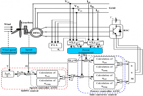
In this study, the topology of the wind energy under study is shown in Figure 1. This type of configuration is a variable speed WT using a DFIG, and also uses a gearbox, but does not require the use of a soft starter or a reactive power compensation. Wind turbines are made up of several mechanical, electrical and control system components. Mechanical components convert the kinetic energy of the wind into mechanical energy, according to physicist Albert Betz.
DFIG converts mechanical energy into electrical energy. As the name suggests, the power of the DFIG is connected to the network through the stator and rotor windings, by means of a power converter. The use of power converters allows flow of the bidirectional power in the rotor circuit and increases the generator speed. In the wind power system, used in this work, a power controller is made to act in cascade with the speed controller, the MPPT system is made to provide the power reference to be followed and, in order to keep the load running smoothly.
Figure 1. Block diagram of the generation system based on DFIG
The WT input power usually is:
${{P}_{v}}=\frac{1}{2}\rho \pi {{R}^{2}}{{v}^{3}}$ (1)
where, r the air density (kg/m3), R is the Radius of WT (m); ν is the wind speed (m/s).
The output mechanical power of WT is:
${{P}_{M}}={{C}_{p}}\text{ }{{P}_{v}}=\frac{1}{2}{{C}_{p}}\left( \lambda ,\text{ }\beta \right)\rho \pi {{R}^{2}}{{v}^{3}}$ (2)
The power coefficient Cp (λ, β) is a non-linear function on the ratio speed of the blades and the wind. This ratio is known as tip speed ratio (TSR).
The TSR is represented by λ and it is defined by:
$\lambda =\frac{{{\Omega }_{t}}R}{v}$ (3)
where, Ωt is the turbine speed (rad/s).
The torque of WT is the ratio of the aerodynamic power to the turbine shaft speed, can be expressed:
${{T}_{M}}=\frac{{{P}_{M}}}{{{\Omega }_{t}}}$ (4)
The generic formula used to model to Cp is reached from curves power of different points of operation turbine.
A numerical approximation that is used to calculate Cp as:
${{C}_{p}}\left( \lambda ,\text{ }\beta \right)=0.5176\left( \frac{116}{{{\lambda }_{i}}}-0.4\beta -5 \right){{e}^{\frac{-21}{{{\lambda }_{i}}}}}+0.0086\lambda $ (5)
${{\lambda }_{i}}=\frac{1}{\lambda +0.08\beta }-\frac{0.035}{1+{{\beta }^{3}}}$ (6)
Figure 2 illustrates the characteristic curves of the power coefficient versus tip speed ratio for different blade angles. As observed, the power coefficient (Cp) changes with blade pitch angle variation. It increases with the decrease in pitch angle and attains its maximum value at a specific value of pitch angle equal to β=0°.
In order to exploit full use of WT power, in low wind speed Cp should be equal to Cp_max=0.48, which is achieved for β=0° and λ=8 [13].
Figure 2. Cp versus λ with angle β
Figure 3. Wind turbine power curve when value of β=0
There is one specific DFIG speed at which the output power of WT is optimal. By the connection of all MPP, the optimal power curve (PM_opt curve) is obtained. The turbine will get the maximum power PM_max, when the wind turbine is in the PM_opt curve (see Figure 3).
Therefore, a Maximum Power Point Tracking (MPPT) control method, which is detailed in the following section, is required to control the rotor speed of the turbine and maintains it at the maximum power.
Finally, the mechanical torque Tm and shaft speed that is injected when generating electricity is affected by the gearbox relationship, and are given by:
$\left\{ \begin{align} & {{T}_{m}}=\frac{{{T}_{M}}}{G} \\ & {{\Omega }_{g}}=\frac{{{\Omega }_{t}}}{G} \\ \end{align} \right.$ (7)
where, Tm the driving torque of the DFIG (N/m), Ωg is the generator shaft speed (rad/s) and G is the gain of gearbox, respectively.
Furthermore, the dynamics of motion of the DFIG-WT coupling is given as follows [14]:
$\frac{d{{\Omega }_{g}}}{dt}=\frac{1}{J}\left( {{T}_{m}}-{{T}_{em}}-f\Omega \right)$ (8)
where, Tem is the electromagnetic torque (N/m), J is the total moment of inertia (Kg.m2) and fv is the coefficient of viscous friction (Kg.m/s).
Maximum Power Point Tracking (MPPT) is a control technique to increase the energy captured and improve the efficiency of energy conversion, many approaches have been discussed in the literature [15]. The MPPT employed in this study relies on the Tip Speed Ratio (TSR) control, which regulates the generator shaft speed continuously, while keeping the TSR at its optimum value (λ=λopt) to capture the maximum wind power. Therefore, the TSR technique consists in determining the speed of the generator which makes it possible to obtain the maximum generated power.
According to the fundamental equation of dynamics making it possible to determine the evolution of the generator speed from the total mechanic torque applied to the rotor, this speed can be adjusted to a reference. This is obtained by using an adequate controller of the speed to have a reference electromagnetic torque [16, 17].
As shown in Figure 4, the MPPT strategy is based on wind speed measurement and speed control needs a controller. Therefore, an anemometer is needed to measure wind speed [18].
From Eq. (3), the optimal WT shaft speed is defined as:
${{\Omega }_{t}}=\frac{{{\lambda }_{opt}}v}{R}$ (9)
According to the gearbox model, the reference DFIG shaft speed is:
${{\Omega }^{*}}_{g}=G\text{ }{{\Omega }_{g}}$ (10)
Figure 4. Wind turbine model and control scheme
The reference electromagnetic torque is obtained from the servo-control of the speed of the generator shaft using a regulator as follows:
${{T}^{*}}_{em}=\operatorname{Re}g\left( {{\Omega }^{*}}_{g}-{{\Omega }_{g}} \right)$ (11)
With Reg: the speed regulator, conventionally a PI controller.
The equations of the generator DFIG of p pairs of poles fed by a set balanced triphasic can then be expressed, in a synchronous rotating d − q frame, as follow [19]:
Stator and rotor voltages:
$\left\{\begin{array}{l}V_{d s}=R_{s} I_{d s}+\frac{d}{d t} \phi_{d s}-\omega_{s} \phi_{q s} \\ V_{q s}=R_{s} I_{q s}+\frac{d}{d t} \phi_{q s}+\omega_{s} \phi_{d s} \\ V_{d r}=R_{r} I_{d r}+\frac{d}{d t} \phi_{d r}-\left(\omega_{s}-\omega\right) \phi_{q r} \\ V_{q r}=R_{r} I_{q r}+\frac{d}{d t} \phi_{q r}+\left(\omega_{s}-\omega\right) \phi_{d r}\end{array}\right.$ (12)
where, Stator and rotor flux:
$\left\{\begin{array}{l}\phi_{d s}=L_{s} I_{d s}+M I_{q s} \\ \phi_{q s}=L_{s} I_{q s}+M I_{q r} \\ \phi_{d r}=L_{r} I_{d r}+M I_{d s} \\ \phi_{q r}=L_{r} I_{q r}+M I_{q s}\end{array}\right.$ (13)
where, Rs and Rr are the resistors of the stator and rotor, respectively; ω=pΩ and ωs are the rotor and stator angular velocity respectively; Ls, Lr, and M are the stator inductance, rotor inductance and mutual inductance, respectively; and p is the number of pole pairs.
The electromagnetic torque can be expressed as a function of the stator flux and rotor currents:
$T_{e m}=\frac{3}{2} p \frac{M}{L_{s}}\left(\phi_{q s} I_{d r}-\phi_{d s} I_{q r}\right)$ (14)
The active and reactive stator powers delivered from the DFIG machine is given by:
$\left\{ \begin{align} & {{P}_{s}}=\frac{3}{2}\left( {{V}_{ds}}{{I}_{ds}}+{{V}_{qs}}{{I}_{qs}} \right) \\ & {{Q}_{s}}=\frac{3}{2}\left( {{V}_{qs}}{{I}_{ds}}-{{V}_{ds}}{{I}_{qs}} \right) \\ \end{align} \right.$ (15)
The adaptation of these equations to the chosen system of axes and to the simplifying assumptions considered in our case gives:
$\left\{\begin{array}{l}\phi_{q s}=0 \\ \phi_{d s}=\Psi_{s}\end{array}\right.$ (16)
$\left\{ \begin{align} & {{V}_{ds}}=0 \\ & {{V}_{qs}}={{V}_{s}}={{\omega }_{s}}{{\Psi }_{s}} \\ \end{align} \right.$ (17)
$\left\{ \begin{align} & {{P}_{s}}=-\frac{3}{2}{{V}_{s}}\frac{M}{{{L}_{s}}}{{I}_{qr}} \\ & {{Q}_{s}}=-\frac{3}{2}{{V}_{s}}\frac{M}{{{L}_{s}}}{{I}_{dr}}+\left( \frac{3{{V}_{s}}^{2}}{2{{L}_{s}}{{\omega }_{s}}} \right) \\ \end{align} \right.$ (18)
Second-order sliding mode control SOSMC is a very attractive suggested solution to improve the performance of SMC sliding modes by increasing accuracy and reducing chattering. The main attribute of SOSMC is the finite time convergence to zero (or to a vicinity of 0) of the sliding variable and its time derivative (S, S') [20].
A number of SOSMC control elements, two of them dedicated to systems of relative degree 2 which are respectively the suboptimal algorithm, the twisting algorithm, and the third is the super twisting algorithm and it is dedicated to systems with dynamics having relative degree 1 with respect to sliding variable S [21].
6.1 Super twisting control STC
The STC is the most effective second-order continuous sliding mode control algorithm. It produces the continuous control function that directs the sliding variable and its derivative to zero (i.e. S=S'=0) in finite time. This algorithm only works with bounded perturbations, therefore a conservative upper bound should be used when designing the controller to ensure that sliding is maintained [22, 23].
We can therefore consider STC algorithm as a nonlinear generalization of a PI controller [24]. The STC algorithm is made of two parts one presents a discontinuity while the other v is continuous [25].
The STC control law expression is given by:
$\left\{ \begin{align} & u={{k}_{1}}{{\left| S \right|}^{r}}sign\left( S \right)+v \\ & \frac{dv}{dt}=-{{k}_{2}}sign\left( S \right) \\ \end{align} \right.$ (19)
where, S and r are the switching function and the exponent, determined respectively defined for the STC controller, and Ki (i=1, 2) are the gains of the proportional and integral parts of the STC controller.
In order to guarantee the convergence of sliding surfaces (S, S') towards zero in a finite time, the gains of the proposed command can be chosen as follows [26]:
$\left\{ \begin{align} & {{k}_{1}}>0 \\ & {{k}_{2}}\ge \frac{4{{A}_{M}}}{{{B}_{m}}^{2}}\frac{{{B}_{M}}\left( {{k}_{1}}+{{A}_{M}} \right)}{{{B}_{m}}\left( {{k}_{1}}-{{A}_{M}} \right)} \\ & 0<r<0.5 \\ \end{align} \right.$ (20)
For a real sliding mode, the control law will be given as follows:
${{u}_{st}}=-{{k}_{1}}{{\left| S \right|}^{0.5}}sign\left( S \right)-\int{{{k}_{2}}sign\left( S \right)}$ (21)
6.2 Adaptive super twisting control ASTC
This is a fairly recent approach, proposed by Shtessel in 2010 and 2012 [27, 28], it consists of using variable control gains that ensure the establishment, in a finite time, of a SOSMC in the presence of limited disturbances by unknown limits. The important feature of the adaptive algorithm is that it does not overestimate the values of the controller’s gains. In this case, the controller gains are variable k1=k1 (s, t) and k2=k2 (s, t). The principle consists in introducing a domain (m³çsê), where once reached, the gains k1and k2 start to decrease dynamically until the trajectories of the system leave this domain, then, these gains start to grow dynamically in order to force these trajectories to return to this domain in finite time. Instead of a fixed gain, ASTC introduces an adaptive gain for the sign function to achieve faster convergence and less chatter. Intuitively, adaptive gain has a low value when the slip function is near zero (where chatter occurs).
Here, we present briefly summarises the ASTC algorithm. Following the notation of Shtessel et al. (2012), the ASTC control law reads [28]:
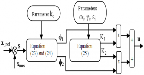
$u=k_{1} \phi_{1}(S)+\int k_{2} \phi_{2}(S)$ (22)
$\phi_{1}(S)=-|S|^{0.5} \operatorname{sign}(S)+k_{c} S$ (23)
$\phi_{2}(S)=\frac{1}{2} \operatorname{sign}(S)+\frac{3}{2} k_{c}|S|^{0.5} \operatorname{sign}(S)+k_{c}^{2} S$ (24)
where, kc>0 is the constant. Values k1=k1 (S, t) and k2=k2 (S, t) are the adaptive gains to be determined.
The control gains k1 and k2 are adapted dynamically according to the ref. [26]:
$\begin{array}{ll}\frac{d k_{1}}{d t}= \begin{cases}\omega_{1} \sqrt{\frac{\gamma_{1}}{2}} \operatorname{sign}(|S|-\mu) & \text { if } k_{1}>0 \\ 0 & \text { if } k_{1}=0\end{cases} \\ k_{2}=2 \varepsilon_{1} k_{1} & \end{array}$ (25)
where, ω1, γ1, μ, ε1> 0, are tunable controller parameters.
Figure 5 shows the block diagram of the proposed controller ASTC.
Figure 5. Block diagram of the proposed ASTC controller
6.3 Application of ASTC control
In this research, the ASTC technique was applied for both MPPT and the power converter control to increase the energy captured from the wind turbine, and to improve power regulation with better efficiency and quality of generated power of WECS. The block diagram of the control system, using the proposed ASTC, is shown in Figure 6.
The inputs of the controllers are the power and speed errors, respectively.
Then, the choice of slip variables is the following:
$\left\{ \begin{align} & {{S}_{d}}={{P}_{s}}^{*}-{{P}_{s}} \\ & {{S}_{q}}={{Q}_{s}}^{*}-{{Q}_{s}} \\ & {{S}_{\Omega }}={{\Omega }^{*}}-\Omega \\ \end{align} \right.$ (26)
Moreover, each component of the action control variables consists of two terms [29].
$\left\{ \begin{align} & {{v}_{d}}={{v}_{d\text{ ast}}}+{{v}_{d\text{ eq}}} \\ & {{v}_{q}}={{v}_{q\text{ ast}}}+{{v}_{q\text{ eq}}} \\ & {{v}_{\Omega }}={{v}_{\Omega \text{ ast}}}+{{v}_{\Omega \text{ eq}}} \\ \end{align} \right.$ (27)
where, the terms with subscript «st» are calculated, through application of the ASTC algorithm, as:
$\left\{ \begin{align} & {{v}_{d\text{ ast}}}={{k}_{1\text{ }d}}\text{ }{{\varphi }_{1\text{ }d}}+\int{{{k}_{2\text{ }d}}\text{ }{{\varphi }_{2\text{ }d}}\text{ }dt} \\ & {{v}_{q\text{ ast}}}={{k}_{1\text{ }q}}\text{ }{{\varphi }_{1\text{ }q}}+\int{{{k}_{2\text{ }q}}\text{ }{{\varphi }_{2\text{ }q}}\text{ }dt} \\ & {{v}_{\Omega \text{ ast}}}={{k}_{1\text{ }\Omega }}\text{ }{{\varphi }_{1\text{ }\Omega }}+\int{{{k}_{2\text{ }\Omega }}\text{ }{{\varphi }_{2\text{ }\Omega }}\text{ }dt} \\ \end{align} \right.$ (28)
With k1and k2 the adaptive gains are expressed as the Eq. (25).
The addends with subscript «eq» in Eq. (27), which correspond to equivalent control terms, can be obtained in a similar way as the traditional SMC, are derived by letting Śd=Śq=ŚΩ=0.
Figure 6. Three-p block diagram of the whole device studied
As a result:
${{v}_{dq\Omega \text{ eq}}}=\left\{ \begin{align} & -\frac{{{L}_{s}}{{L}_{r}}\sigma }{M{{V}_{s}}}\overset{\bullet }{\mathop{{{Q}_{s}}^{*}}}\,+{{R}_{r}}{{I}_{d\text{r}}} \\ & -\frac{{{L}_{s}}{{L}_{r}}\sigma }{M{{V}_{s}}}\overset{\bullet }{\mathop{{{P}_{s}}^{*}}}\,+{{R}_{r}}{{I}_{q\text{r}}}+g\frac{M{{V}_{s}}}{{{L}_{s}}} \\ & {{T}_{m}}-f\Omega -J\frac{d}{dt}{{\Omega }^{*}} \\ \end{align} \right.$ (29)
Equivalent control terms are therefore included not only to improve the transient response of the system, but also for the adjustment of the ASTC gains αi and βi.
To test and analyze the performances of the proposed control strategy using the controllers based on Super-Twisting Adaptive, simulations were carried out using the complete dynamic model of Figure 6. The Simulation has been realized using Matlab–Simulink software with a 1.5 (MW)DFIG coupled to a grid [30].
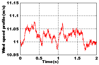
The temporal evolution of the wind used in this simulation is shown in Figure 7. Representative results obtained by simulation during 2s of the controlled system with each of the designed controllers are presented and analyzed below.
Figure 7. Wind speed profile
DFIG-WT parameters values are listed below in Table 1 in appendix.
Table 1. DFIG-wind turbine parameters
|
Parameter |
Value |
Unity |
|
DFIG |
||
|
Nominal power |
1.5 |
MW |
|
Nominal voltage |
690 |
V |
|
Frequency |
50 |
Hz |
|
Poles pairs number |
2 |
- |
|
Stator resistance |
2.65.10-3 |
Ω |
|
Rotor resistance |
2.63.10-3 |
Ω |
|
Stator inductance |
5.60.10-3 |
H |
|
Rotor inductance |
5.60.10-3 |
H |
|
Mutual inductance |
5.48.10-3 |
H |
|
Turbine |
||
|
Number of blades |
3 |
- |
|
Air density |
1.225 |
Kg/m3 |
|
Turbine radius |
35.25 |
M |
|
Gearbox ratio |
75 |
- |
|
DFIG+ Turbine |
||
|
Generator inertia |
1000 |
Kg.m2 |
|
Friction factor |
0.0024 |
Kg.m/s |
Table 2. STC controller parameters
|
Speed controller |
Power controller |
|
K1Ω=1.5sqrt(L) |
K1=1.5sqrt(L) |
|
K2Ω=1.1(L) |
K2=1.1(L) |
|
L=500 |
L=15000 |
Table 3. ASTC controller parameters
|
Speed controller |
Power controller |
|
kc=120 |
kc=500 |
|
Ω1=20 |
ω1=60 |
|
Γ1=1 |
γ1=1 |
|
m1=0.05 |
m1=0.005 |
|
ε1=2 |
ε1=10 |
Moreover, the ASTC controller’s settings were used shown above in Table 2, and for the STC controllers, the fixed gains can be chosen as shown in Table 3.
7.1 MPPT responses
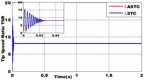
Figure 8 illustrates the dynamic performance of the WT system obtained by using two different control schemes, we note respectively from top to bottom the aerodynamic power obtained, the variation of the speed ratio and the variation of the coefficient of power.
(a) T reference active power Ps*
(b) Tip speed ratio TSR
(c) Power coefficient Cp
Figure 8. Comparison of the performance of wind turbine system
Figure 8(a) presents the reference stator active power with MPPT process, which the DFIG-WT proves an optimum capacity operation.
It can be seen in Figure 8(b) and Figure 8(c) that the MPPT strategy ensures the tracking of the optimum power points, by maintaining the coefficient of performance around its maximum, and the TSR around its optimum value. From these figures, the smoothness of the proposed ASTC is proved, and this is responsible for improved mechanical behavior. The simulation results show that the proposed control scheme for MPPT control of the WT presents better performances in capturing the optimal wind energy as well as chattering suppression.
7.2 Whole system responses
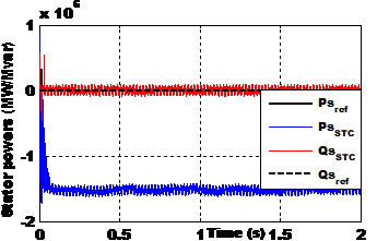
Figure 9 shows a comparison of stator active and reactive powers response of DFIG, PS, and QS, together with the optimal powers PS* and QS*, for the controlled system with each of the designs developed. While Figure 9(a) corresponds to the adaptive ASTC controller, Figure 9(b) presents the curves corresponding to the system controlled by the conventional STC. It can be observed from this figure that despite the variation in wind speed and machine parameters, the active and reactive powers of the DFIG accurately follow their reference values for both schemes, but with a smaller error and oscillation for ASTC in steady-state. On the other hand, we also see in the event of a reference shift that the ASTC does not have any overshoot of the two powers during the transient phenomenon, this implies an attenuation of the oscillations. In Figures 10(a) and 10(b), the detail of the oscillations and the resulting chattering of the STC controller are shown.
Moreover, the spectral analysis of the line current illustrated in Figures 11(a) and 11(b) clearly shows that the total harmonic distortion was minimized by almost a third for the ASTC controller (THD=0.21%) compared to the STC controller (THD=0.62%).
(a) With ASTC controller
(b) With STC controller
Figure 9. Powers response comparison
(a) Active powers
(b) Reactive powers
Figure 10. Powers zoom of comparison power responses
(a) With ASTC controller
(b) With STC controller
Figure 11. Spectrum harmonic of one phase stator current
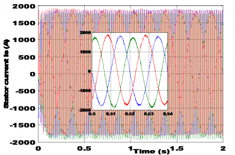
The three-phase currents obtained from the stator using ASTC scheme represented in Figure 12(a) shows that they have sinusoidal shapes less wavy than using STC scheme in Figure 12(b), which signifies clean energy without harmonics supplied to the network. Finally, Figure 13(a) and Figure 13(b) show the rotor currents drawn by DFIG using ASTC control and conventional STC respectively. It is clear that the frequency of the rotor currents is lower than the frequency of the stator currents.
(a) With ASTC controller
(b) With STC controller
Figure 12. Three- phase stator currents of the DFIG
(a) With ASTC controller
(b) With STC controller
Figure 13. Three- phase rotor currents of the DFIG
In this work, an adaptive no-linear control algorithm based on sliding mode is developed to improve the control strategy of DFIG driven by a wind energy conversion system, under variable wind speed and connected to the electrical network. This method combines the advantages of second-order super-twisting sliding mode control and the adaptive control methodology.
The proposed control scheme using ASTC Controllers guarantees an efficient performance for tracking time-varying references generated by the Tip Speed Ratio MPPT control algorithm, to extract the maximum power under wind speed turbulence.
At the same time, the regulation of the active power, as well as the reactive power, is carried out efficiently, which contributes to a correct control of the wind energy conversion system with better-generated power quality.
The design of ASTC controllers’ parameters has an impact on control performance and has to be adequately chosen. As such, future work will focus on tuning the proposed controller’s parameters using optimization techniques to find their optimal values in an auto-manner and to demonstrate the feasibility of the proposed approaches by the development of a prototype to experimentally validate the proposed control method.
[1] Arturo Soriano, L., Yu, W., Rubio, J.D.J. (2013). Modeling and control of wind turbine. Mathematical Problems in Engineering, 2013. https://doi.org/10.1155/2013/982597
[2] Zaid, M.M., Ro, J.S. (2019). Switch Ladder modified H bridge multilevel inverter with novel pulse width modulation technique. IEEE Access, 7: 102073-102086. https://doi.org/10.1109/ACCESS.2019.2930720
[3] Wu, B., Lang, Y., Zargari, N., Kouro, S. (2011). Power Conversion and Control of Wind Energy Systems. John Wiley & Sons.
[4] Djeriri, Y., Meroufel, A., Allam, M. (2015). Artificial neural network-based robust tracking control for doubly fed induction generator used in wind energy conversion systems. Journal of Advanced Research in Science and Technology, 2(1): 173-181. https://doi.org/10.13140/RG.2.1.3750.120
[5] Barambones, O., Cortajarena, J.A., Alkorta, P., De Durana, J.M.G. (2014). A real-time sliding mode control for a wind energy system based on a doubly fed induction generator. Energies, 7(10): 6412-6433. https://doi.org/10.3390/en7106412
[6] Kunusch, C., Puleston, P., Mayosky, M. (2012). Sliding-Mode Control of PEM Fuel Cells. Springer Science & Business Media. https://doi.org/10.1007/978-1-4471-2431-3
[7] Martinez, M.I., Tapia, G., Susperregui, A., Camblong, H. (2012). Sliding-Mode control for DFIG rotor- and grid-side converters under unbalanced and harmonically distorted grid voltage. IEEE Transactions on Energy Conversion, 27(2): 328-339. https://doi.org/10.1109/tec.2011.2181996
[8] Moussa, O., Abdessemed, R., Benaggoune, S., Benguesmia, H. (2018). Power quality enhancement grid connected brushless doubly-fed induction generator using sliding mode control. The 6th International Conference on Mechanics and Energy ICME, Hamamaet, Tunisia. https://doi.org/10.18280/ejee.210504
[9] Tang, C.Y., Guo, Y., Jiang, J.N. (2011). Nonlinear dual-mode control of variable-speed wind turbines with doubly fed induction generators. IEEE Transactions on Control Systems Technology, 19(4): 744-756. https://doi.org/10.1109/TCST.2010.2053931
[10] Levant, A., Shustin, B. (2018). Quasi-Continuous MIMO sliding-mode control. IEEE Trans. Autom. Control, 63: 3068-3074. https://doi.org/10.1109/TAC.2017.2778251
[11] Han, Y., Li, S., Du, C. (2020). Adaptive higher-order sliding mode control of series-compensated DFIG-based wind farm for sub-synchronous control interaction mitigation. Energies, 13(20): 5421. https://doi.org/10.3390/en13205421
[12] Benchagra, M., Maaroufi, M., Ouassaid, M. (2012). Nonlinear MPPT control of squirrel cage induction generator-wind turbine. Journal of Theoretical and Applied Information Technology, 35(1): 26-33.
[13] Boubzizi, S., Abid, H., El hajaji, A., Chaabane, M. (2018). Adaptive super-twisting sliding mode control for wind energy conversion system. International Journal of Applied Engineering Research, 13(6): 3524-3532.
[14] Fuchs, F., Mertens, A. (2012). Dynamic modelling of a 2 MW DFIG wind turbine for converter issues: Part 1. In 2012 15th International Power Electronics and Motion Control Conference (EPE/PEMC), pp. DS2d.5-1-DS2d.5-7. https://doi.org/10.1109/EPEPEMC.2012.6397308
[15] Abdeddaim, S., Betka, A. (2013). Optimal tracking and robust power control of the DFIG wind turbine. International Journal of Electrical Power & Energy Systems, 49: 234-242. https://doi.org/10.1016/j.ijepes.2012.12. 7916014
[16] Lei, Z., Sun, X., Xing, B., Hu, Y., Jin, G. (2018). Active disturbance rejection based MPPT control for wind energy conversion system under uncertain wind velocity changes. Journal of Renewable and Sustainable Energy, 10(5): 053307. https://doi.org/10.1063/1.503
[17] Thongam, J.S., Ouhrouche, M. (2011). MPPT control methods in wind energy conversion systems. Fundamental and Advanced Topics in Wind Power, 15: 339-360. https://doi.org/10.5772/21657
[18] Yaichi, I., Semmah, A., Wira, P. (2020). Control of doubly fed induction generator with maximum power point tracking for variable speed wind energy conversion systems. Periodica Polytechnica Engineering and Computer Science, 64(1): 78-96. https://doi.org/10.3311/PPee.14166
[19] Amer, M., Miloudi, A., Lakdja, F. (2020). Optimal DTC control strategy of DFIG using variable gain PI and hysteresis controllers adjusted by PSO algorithm. Periodica Polytechnica Electrical Engineering and Computer Science, 64(1): 74-86. https://doi.org/10.3311/PPee.14237
[20] Benelghali, S., Benbouzid, M.E.H., Charpentier, J.F., Ahmed-Ali, T., Munteanu, I. (2011). Experimental validation of a marine current turbine simulator: Application to a PMSG-based system second-order sliding mode control. IEEE Trans. Industrial Electronics, 58(1): 118-126. https://doi.org/10.1109/TIE.2010.2050293
[21] Beltran, B., Benbouzid, M.E., Ahmed-Ali, T. (2012). Second-order sliding mode control of a doubly fed induction generator driven wind turbine. IEEE Transactions on Energy Conversion, 27(2): 261-269. https://doi.org/10.1109/TEC.2011.2181515
[22] Rafiq, M., Rehman, S., Rehman, F., Butt, Q.R., Awan, I. (2012). A second order sliding mode control design of a switched reluctance motor using super twisting algorithm. Simulation Modelling Practice and Theory, 25: 106-117. https://doi.org/10.1016/j.simpat.2012.03.001
[23] Yaichi, I., Semmah, A., Wira, P., Djeriri, Y. (2019). Sliding super-twisting sliding mode control of a doubly-fed induction generator based on the SVM strategy. Periodica Polytechnica Engineering and Computer Science, 63(3): 178-190. https://doi.org/10.3311/PPee.13726
[24] Kahal, H., Taleb, R., Boudjema, Z., Bouyekni, A. (2017). Super twisting sliding mode control of dual star induction generator for wind turbine. The Mediterranean Journal of Measurement and Control, 13(3): 788-794.
[25] Borlaug, I.L.N. (2017). Higher-order sliding mode control. Master of Science in Cybernetics and Robotics. Norwegian University of Science and Technology, Department of Engineering Cybernetics.
[26] Listwan, J. (2018). Application of super-twisting sliding mode controllers in direct field-oriented control system of six-phase induction motor: Experimental studies. Power Electronics and Drives, 3(1): 23-34. https://doi.org/10.2478/pead-2018-0013
[27] Shtessel, Y.B., Moreno, J.A., Plestan, F., Fridman, L.M., Poznyak, A.S. (2010). Super-twisting adaptive sliding mode control: A Lyapunov design. 49th IEEE Conference on Decision and Control (CDC) - Atlanta, GA, USA, pp. 5109-5113. https://doi.org/10.1109/CDC.2010.571790
[28] Shtessel, Y., Taleb, M., Plestan, F. (2012). A novel adaptive gain super twisting sliding mode controller. Methodology and application. Automatica, 48(5): 759-769. https://doi.org/10.1016/j.automatica.2012.02.024
[29] Ouaria, K., Rekioua, T., Ouhrouche, M. (2012). Real time simulation of nonlinear generalized predictive control for wind energy conversion system with nonlinear observer. ISA Transactions, 53(1): 76-84. https://doi.org/10.1016/j.isatra.2013.08.004
[30] Evangelista, C., Valenciaga, F., Puleston, P. (2013). Active and reactive power control for wind turbine based on a MIMO 2-sliding mode algorithm with variable gains. IEEE Transactions on Energy Conversion, 28(3): 682-689. https://doi.org/10.101610.1109/TEC.2013.2272244