Amri Omar* | Fri Mohamed | Msaaf Mohammed | Belmajdoub Fouad
© 2021 IIETA. This article is published by IIETA and is licensed under the CC BY 4.0 license (http://creativecommons.org/licenses/by/4.0/).
OPEN ACCESS
The elaboration and development of monitoring (diagnostic and prognostic) tools for industrial systems has been one of the main concerns of the researchers for many years, so that many researches and studies have been developed and proposed, especially concerning discrete event systems (DES), which occupy an important class of industrial systems. However, the use of modeling tools to ensure these operations become a complex and exhausting task, while the complexity of industrial systems has been increasing incessantly. Therefore, the development of more and more sophisticated techniques is required. In this context, the use of artificial neural networks (NN) seems interesting, because thanks to their automatics and intelligent algorithms, the NN could handle perfectly DES diagnosis and prognosis problems. For this purpose, in the following papers, we propose an intelligent approach based on feed-forward neural network, which will deal with fault diagnosis and prognosis in DES, so that the events generated by the DES, will be presented and analyzed by the neural network in real-time, in order to perform an online diagnosis and prognosis.
industrial systems, monitoring tools, discrete event systems, faults diagnosis, faults prognosis, feed-forward neural networks
The industrial world never ceases to develop, which creates an important competitiveness in the market and pushes the industries to optimal exploitation of their means, not only equipment but also human resources [1]. In this context, the efficiency of the maintenance function of the industrial systems has become one of the big challenges so that it is no longer considered an expensive expense item. Contrarily, it is now identified as a major and a profits-making function [2], so that the fact of keeping the equipment in their optimal state during the production, has become a fundamental point of the product and the company’s success.
Every system is supposed to comfort different types of defects, which can lead to a radical change in the normal behavior of the process and sometimes to a degradation of its performance, in such a way that it can no longer fulfil and accomplish its function. In this sense, diagnosis or fault detection and prognosis or fault prevention, which is considered a very important phase of maintenance, so that the more efficient the diagnosis and prognosis, the more effective the operations and maintenance interventions are, is necessary to prevent the propagation of breakdowns and limit their consequences that can affect the availability, reliability, and safety of equipment, by taking many actions either preventives or correctives one [3]. This problem has attracted the attention of the scientific community for several years, so that much research has been developed, mainly concerning discrete event systems (DES), which occupy several fields of application in different industries. About DES, the approaches based on models are usually used to ensure the diagnosis and prognosis operation, in particular finite automata [4, 5], Petrie net [6, 7], and their extensions [8-10]. The use of such tools is generally confronted by various stumbling blocks and difficulties, namely the model development and the difficulty of implementation, in addition that the systems are generally subject to a permanent reconfiguration and adaptation to their environment [11]. Therefore, the use of artificial intelligence techniques presents an obvious interest for the industries, especially since the word is explicitly heading toward the so-called maintenance 4.0 instead of a classic one. The aim of this research is the exploitation of artificial neural networks, which can deal with high learning capacity and great flexibility to progress in a dynamic context [11], to ensure the DES diagnosis and prognosis, based on the statistical model of the desired system. Moreover, in the literature, neural networks are generally reserved to the continuous system and the use of such tools for the benefit of DES is very limited [12, 13].
The rest of these papers is organized as follows: In section 2, a general context and basic definitions and notions concerning DES and its fault diagnosis and prognosis are presented, we also highlight the way to ensure these functions using feed-forward neural networks. In section 3, an approach to ensure DES fault’s diagnosis and prognosis using feed-forward neural networks and its theoretical framework in addition to sufficient and necessary conditions for diagnosability and prognosability are presented, and based on the results obtained in section 3, a learning database to train the neural networks in order to achieve the desired operations is constructed. Eventually, and in order to determine and prove the relevance of the approach proposed, a case study on a real discrete event system is presented.
2.1 Definitions
A discrete event system (DES) is a system, which the transformation or the evolution of states is launched by the occurrence of point events, typically the arrival of signal or the completion of a task [14, 15]. The word discrete does not mean discrete-time or discrete state, but it refers to the dynamic is composed of events, which can be the beginning and the end of continuous evolution. So, a DES can be considered as a generator of events ∑ [4], so that each event leads to specific state. ∑ is named by “Alphabet” and it is considered as a set of events that can be generated by the DES, either they are observed or not i.e., ∑ can be divided to two main categories [16]:
●Observable events noted by $\sum_{o}$ such as $\sum_{o}=\left\{e_{1}, e_{2}, \ldots, e_{N}\right\}$ so that their occurrence can be observed and recorded.
●Unobservable events noted by $\sum_{uo}$, which may be failure events $\sum_{f}$ or regular events $\sum_{r}$ that can deviate the DES from a normal functioning to a faulty one. Such as $\sum_{u o}=\sum_{f} \cup \sum_{r}$, where $\sum_{r}=\left\{r_{1}, r_{2}, \ldots, r_{m}\right\}$ is the set of regular events and $\sum_{f}=\left\{f_{1}, f_{2}, \ldots, f_{\alpha}, \ldots, f_{p}\right\}$ is the set of unobservable events, which can be a fault such as the set of failure $\sum_{f}$ is corresponded to the different failures that the DES may come across to them. Therefore, for the alphabet ∑ we can write that: $\sum=\sum_{o} \cup \sum_{f} \cup \sum_{r}=\sum_{o} \cup \sum_{u o}$.
Generally, a DES operates in cycles called functioning cycle and each one deal with different tasks to achieve a predetermined state. Each functioning cycle is noted by “σ” and it is composed by a sequence of events, which can be observable or unobservable forming a finite timed word (we note the set of all the timed words that can be generated by a DES by TW*) [16] so that each event is indexed by its occurrence time e.g. $\sigma=e_{1}^{t_{1}} e_{2}^{t_{2}} \ldots e_{i}^{t_{i}} \ldots e_{k}^{t_{k}}$ is a finite timed word such as ei is an event belonging to ∑ and ti is its time of occurrence [17], so that $t_{i} \in \mathbb{R}^{+}$. They are several approaches to represent time in a finite timed word, the most common is the one presented in [18, 19]. In this representation, instead of indexing the events with their times of occurrence, the authors suggest coupling the events with time between their proper occurrence and the occurrence of the previous event. In this case, given a $\sigma=e_{1}^{t_{1}^{\prime}} e_{2}^{t_{2}^{\prime}} \ldots e_{i}^{t_{i}^{\prime}} \ldots e_{k}^{t_{k}^{\prime}}, t_{i}^{\prime}=t_{i}-t_{i-1}$.
2.2 DES diagnosis and prognosis
Diagnosis or fault location is the process of determining if a fault has occurred in the system or not, as well as locating its location, i.e., the diagnosis aim to detect a deviation from the normal and nominal behavior of the system as early as possible and to determine the causes and the consequences [20, 21]. The diagnosis is composed of three main phases [20, 22]:
● $1^{ {st }} phase$ : Consists in detecting the occurrence of an anomaly i.e., to decide either the system works in normal and nominal conditions or a fault has occurred.
● $2^{ {nd }} phase$ : Consists in locating this anomaly and looking for the causes i.e., if a fault has occurred (Detected at the first phase), fault location aims at localizing the component(s) and the element(s) of the system causing the fault.
● $3^{ {rd }} phase$ : Consists in analyzing the consequences of the anomaly on the overall system i.e., to analyze all possible effects of the anomaly on all sides (its criticality, importance, etc.).
In DES context, the diagnosis consists of detecting the occurrence of a faulty event $f_{\alpha} \in \sum_{f}$, and specified its location over the observable events generated by the DES.
Prognosis or fault prediction is the operation that predicts the behavior and the state of a system in the future, i.e., anticipating the appearance of anomalies over time intervals extending from the instance a prediction is made to the instance of the appearance of an anomaly leading the system to deviate from its normal behavior to a faulty one [21]. Concerning DES prognosis, it consists of the prediction of the occurrence of a faulty event $f_{\alpha} \in \sum_{f}$ and determining the remaining time before that this event may appear in order to take the necessary actions to ensure the proper functioning of the system.
2.3 Fault diagnosis and prognosis using neural networks
Neural Network (NN) is a tool of artificial intelligence widely used to solve a variety of problems so that their progress extends to several industries and applications [23]. Because, thanks to their learning capacity, they are used to solve the most complex problems in several fields. This capacity is the result of an intelligent process called learning or training. The main role of this process is: Based on a set of data presented to the neural network, it establishes a relation between the set of inputs and the set of outputs in order to take advantage and generalizes the obtained knowledge during training to new sets of data [24]. A neural network is generally formed by nodes organized in layers, which can be divided into three types: input, hidden, and output layer. So that each node can be connected to the node of the successor layer, in the case of feed-forward neural networks, or can be linked to any other nodes even to itself, in the case of recurrent neural networks [25].
The purpose of this research is to use feed-forward neural networks in order to determine the probable current state of the DES (Diagnosis) by detecting either a faulty event $f_{\alpha} \in \sum_{f}$ is generated or not, as well as identify the probable future state of the DES (Prognosis) by detecting either a faulty event $f_{\alpha} \in \sum_{f}$ can be generated in the future functioning of the DES or not. Therefore, the main approach to analyze and exploit the event generated by the DES using feed-forward neural networks, which can deal in the same time with the diagnosis and the prognosis, is to use Temporal window or Spatio-temporal representation [16] so that, this technique can be used for any feed-forward neural network architecture or type. The idea behind this approach is: Instead of presenting to the neural network each event generated by the DES as it occurs. It has to wait until a number of event “q”, which depend necessarily on the problem treated, has occurred i.e., to delay the events a certain time before presenting them to the NN and each temporal delay represent a dimension of the temporal window, so that for each temporal window presented to the NNs, the NNs provide the probability that a faulty event has appeared in the temporal window on the case of diagnosis and the probability that a faulty event may appear after the occurrence of the temporal window in addition to the remaining time before a fault in the case of prognosis. They are several research, which use this technique, we can find those presented in the references [26, 27] where the authors used a spatial time representation for speech processing, also other research presented in the references [16, 28]. The following Figure 1 shows how the diagnosis and prognosis can be done using temporal window:
Figure 1. Diagnosis and prognosis using feed-forward neural networks
In practice, the use of this method shows several limits: Firstly, to ensure the functions of diagnosis and prognosis it is necessary to define the size of the temporal window, which will determine the number of neural networks inputs that directly modifies the NN architecture and structure as well as its performance and response time, which can be very important [29]. More, if the size of the temporal window is large, the diagnosis and prognosis cannot be operational at the beginning of the DES functioning, because we have to wait until the occurrence of “q” events to form a temporal window and start the diagnosis and prognosis. Furthermore, by using temporal windows, it is not possible to determine the exact location of the occurrence of an unobservable, i.e., to exactly determine between which observable events an unobservable event has occurred, which does not allow accomplishing the second phase of the diagnosis, which consists on exactly locating the location of the abnormality. Moreover, if two temporal windows are more or less similar, the NNs may not distinguish between them and treat them in the same way [30]. Therefore, in these papers, in order to solve the problems above and mitigate these limits, we propose a new approach, its aim is instead of diagnosing and prognosing temporal windows, we will use temporal pairs i.e., two successive observable events. In such a way to use it to compute the probability that an unobservable event has occurred between two successive observable events (diagnosis) and also compute the probability that an unobservable event can be generated during the next DES functioning states (prognosis). By using this approach, we will have the ability to distinguish exactly the location where an unobservable has occurred. Moreover, we will not worry about the complexity of the neural network architecture, which can deal with the best results, because by using just two events as NNs inputs, the size of the input vectors is much more minimized, comparing it with the temporal windows, which usually contain a large number of events, which results to a more efficient training of the NNs. In addition, we will have the possibility to launch the diagnosis and prognosis from the first two events generated by the system. Concerning the problem of the similarity, which can be also between the temporal pairs, the solution proposed will be presented and analyzed in details in the next sections.
The most important phase in the neural network building is the training phase, where a set of data containing the inputs and their corresponding outputs is presented to the NN in order to generalize the knowledge taken from these data to new on. Therefore, to ensure DES diagnosis and prognosis the first step is to build a statistical model of the DES, which is considered as a database containing the description of all the possible behaviors (normal and abnormal) of the desired system in form of historical data for each possible functioning cycle $\sigma^{j} \in T W^{*}$, in both normal and faulty states. Such as $\sigma^{j}$ is the jth functioning cycle according to the DES can operate.
Definition 1 (A temporal pair from a timed word): We consider a timed word $\sigma_{j^{\prime}}^{j} \in T W^{j *}$ (such as $T W^{j *}$ the set of all the historical data, which concern the functioning cycle j) so that $\sigma_{j^{\prime}}^{j}=e_{1}^{t_{1}} e_{2}^{t_{2}} \ldots e_{i}^{t_{i}} \ldots e_{k}^{t_{k}}$ recorded from the $j^{\prime t h}$ cycle of a DES according to the jth functioning cycle and ‘k’ is the number of observable events. A temporal pair is a couple of observable events i.e., two successive events generated by the DES, more formally: $T P_{j^{\prime}.i}^{j}=e_{i-1}^{t_{i-1}} e_{i}^{t_{i}}$, so that $T P_{j^{\prime}.i}^{j}$ is the ith temporal pair derived from a $\sigma_{j \prime}^{j}$, and contain two successive observable events.
Given Tp a temporal pair, we consider the following notation:
● $P_{o}(T p): T p \rightarrow \sum_{o}$: the projection, which eliminate time and unobservable events from a temporal pair in the case that they exist.
● $P_{u}(T p): T p \rightarrow \sum_{f}$: the projection that keep just unobservable events from a temporal pair and remove observable events and time.
● $T(T p): T p \rightarrow \mathbb{R}^{+}$: the projection, which gives the occurrence time of each event in Tp.
● $S_{j^{\prime}}^{j}$: The set of all temporal pairs derived from a $\sigma_{j \prime}^{j}$.
● $S_{j^{\prime} f_{\alpha}}^{j}(T p)$: the set of all temporal pairs derived from a $\sigma_{j \prime}^{j}$ and has the same projection as Tp as well as contain a faulty event $f_{\alpha} \in \sum_{f}$ more formally:
$S_{j^{\prime} f_{\alpha}}^{j}(T p)=\left\{T P_{j^{\prime} . i}^{j} \in S_{j^{\prime}}^{j} / P_{o}\left(T P_{j^{\prime}.i}^{j}\right)=T p P_{u}\left(T p_{j^{\prime}.i}^{j}\right)=f_{\alpha}\right\}$
● $S_{j^{\prime}}^{j}(T p)$: the set of all temporal pair derived from a $\sigma_{j \prime}^{j}$, which has the same projection as Tp more formally:
$S_{j^{\prime}}^{j}(T p)=\left\{T P_{j^{\prime}.i}^{j} \in S_{j^{\prime}}^{j} / P_{o}\left(T P_{j^{\prime}.i}^{j}\right)=T p\right\}$
Example 1: We consider a DES defined by their sets $\sum=\left\{a, b, c, d, f_{1}, f_{2}, f_{3}, r_{1}, r_{2}\right\}$ partitioned into the following sets of events $\sum_{o}=\{a, b, c, d\}, \sum_{f}=\left\{f_{1}, f_{2}, f_{3}\right\}$ and $\sum_{ {reg }}=\left\{r_{1}, r_{2}\right\}$, such as the events $f_{1}, f_{2}, f_{3}$ correspond to a faults, which should be diagnosed and prognoses. We consider $\sigma_{1}^{1}$ a timed word generated by the DES during the first cycle according to the first functioning cycle, so that:
$\sigma_{1}^{1}=b^{1} a^{1,5} f_{1}^{2,3} c^{4} b^{5} f_{2}^{5,6} a^{7} r_{1}^{7,3} d^{9,1} f_{1}^{9,3} c^{11} b^{12} a^{12,4} f_{3}^{12,9} c^{13,1} b^{14}$
So that a,b,c and d are the DES observable events, $f_{1}, f_{2}, f_{3}$ correspond to the faulty events, and $r_{1}, r_{2}$ are the DES regular events, in addition, that each event is endowed by its occurrence time.
Then:
$S_{1}^{1}=\left\{\begin{array}{c}T p_{1.1}^{1}=b^{1} a^{1,5}, T p_{1.2}^{1}=a^{1,5} f_{1}^{2,3} c^{4}, T p_{1.3}^{1}=c^{4} b^{5}, T p_{1.4}^{1}=b^{5} \\ f_{2}^{5,6} a^{7}, T p_{1.5}^{1}=a^{7} r_{1}^{7,3} d^{9,1}, T p_{1.6}^{1}=d^{9,1} f_{1}^{9,3} c^{11}, T p_{1.7}^{1}=c^{11} b^{12} \\ T p_{1.8}^{1}=b^{12} a^{12,4}, T p_{1.9}^{1}=a^{12,4} f_{3}^{12,9} c^{13,1}, T p_{1.10}^{1}=c^{13,1} b^{14}\end{array}\right\}$
Concerning $S_{j^{\prime}}^{j}(T p)$ and $S_{j^{\prime} f_{\alpha}}^{j}(T p)$ we take Tp=ba as example, so we obtain: $S_{1}^{1}(b a)=\left\{T p_{1.1}^{1}, T p_{1.4}^{1}, T p_{1.8}^{1}\right\}$ and $S_{1 f_{2}}^{1}(b a)=\left\{T p_{1.4}^{1}\right\}$.
But we can clearly observe that a temporal pair Tp can occur several times in different phases when a timed word is generated by the DES (The disadvantages already discussed in the previous section), therefore, each one of them must be diagnosed and prognoses separately, in such a way, we can accurately define the various behaviors of the DES. For this reason, we propose to split each timed word into sub timed words or rows (r), so that each sub timed word represents a functioning phase with respect to a $\sigma_{j \prime}^{j}$ and this partition will be done in such a way that a sub timed word must not contain temporal pairs with the same projection Po.
Remarque 2: The index (r) will be also another neural network input, which will be incremented automatically, in addition to the functioning cycle index (j) and the current temporal pair in order to give the neural network the ability to distinguish in which phase and functioning cycle the DES is working, and which allow to the neural network in the same time to exhibit a dynamic behavior.
For this purpose, we will define a new set $S_{j^{\prime} . r}^{j}$, which will be the set of all the temporal pairs derived from a cycle $\sigma_{j^{\prime}}^{j} \in T W^{j *}$ and belong to the same sub-timed word “r”.
Example 2: Let us consider again $\sigma_{1}^{1}$ from the previous example, the sub timed words derived from it will be as follow:
$S_{1.1}^{1}=\left\{T p_{1.1}^{1}=b^{1} a^{1,5}, T p_{1.2}^{1}=a^{1,5} f_{1}^{2,3} c^{4}, T p_{1.3}^{1}=c^{4} b^{5}\right\}$,
$S_{1.2}^{1}=\left\{T p_{1.4}^{1}=b^{5} f_{2}^{5,6} a^{7}, T p_{1.5}^{1}=a^{7} r_{1}^{7,3} d^{9,1}, T p_{1.6}^{1}=\right.$$\left.d^{9,1} f_{1}^{9,3} c^{11}, T p_{1.7}^{1}=c^{11} b^{12}\right\}$,
$S_{1.3}^{1}=\left\{T p_{1.8}^{1}=b^{12} a^{12,4}, T p_{1.9}^{1}=a^{12,4} f_{3}^{12,9} c^{13,1}, T p_{1.10}^{1}\right.$$\left.=c^{13,1} b^{14}\right\}$.
3.1 Diagnosability
In the literature, they are several definitions of diagnosability, the most common is the one proposed by Sampath et al. [4], which they define diagnosability of a DES as the ability to detect with a finite delay the occurrences of certain distinguished unobservable events, namely the failure events. In the case of temporal pairs, we define the diagnosability, as the capacity to detect the occurrence of a faulty event $f_{\alpha} \in \sum_{f}$ between two successive observable events and we say a temporal pair is diagnosable if we can detect with certainty its occurrence. So, to ensure this operation, we define an index, similar to the one defined in [8], called the diagnosability index noted by $P_{r}^{j}\left(f_{\alpha} / T p\right)$, which is a statistical index that allows computing the probability that a faulty event $f_{\alpha} \in \sum_{f}$ occurs between two successive observable events generated by the DES, based on the historical data and the statistical model collected for the functioning cycle $\sigma^{j}$ in the row “r” of the desired DES, so that:
$P_{r}^{j}\left(f_{\alpha} / T p\right)=\frac{\sum_{j^{\prime}} \operatorname{card}\left(S_{j^{\prime} f_{\alpha}}^{j}(T p) \cap S_{j^{\prime}. r}^{j}\right)}{\sum_{j^{\prime}} {card}\left(S_{j^{\prime}}^{j}(T p) \cap S_{j^{\prime}. r}^{j}\right)}$
where: $S_{j^{\prime} f_{\alpha}}^{j}(T p) \cap S_{j^{\prime} \cdot r}^{j}$ is the set of all temporal pairs similar to Tp and belong to the sub-timed word “r” and contain the faulty event $f_{\alpha}$. And $S_{j^{\prime}}^{j}(T p) \cap S_{j^{\prime}. r}^{j}$ is the set of all temporal pairs similar to Tp, which belong to the sub timed word “r”. So that $0 \leq P_{r}^{j}\left(f_{\alpha} / T p\right) \leq 1$. And we say Tp is diagnosable with respect to faulty event $f_{\alpha}$ if $P_{r}^{j}\left(f_{\alpha} / T p\right)=1$ or $P_{r}^{j}\left(f_{\alpha} / T p\right)=0$.
Proof:
●In the case of $P_{r}^{j}\left(f_{\alpha} / T p\right)=1$:
$P_{r}^{j}\left(f_{\alpha} / T p\right)=1 \Leftrightarrow \sum_{j^{\prime}} \operatorname{card}\left(S_{j^{\prime} f_{\alpha}}^{j}(T p) \cap S_{j^{\prime} \cdot r}^{j}\right)=$
$\sum_{j^{\prime}} \operatorname{card}\left(S_{j^{\prime}}^{j}(T p) \cap S_{j^{\prime} \cdot r}^{j}\right) \Leftrightarrow \forall \sigma_{j^{\prime}}^{j} \in T W^{j *}, \forall T p_{j^{\prime} \cdot i}^{j} \in$
$S_{j^{\prime} \cdot r}^{j}: P_{o}\left(T p_{j^{\prime}. i}^{j}\right)=T p \Rightarrow P_{u}\left(T p_{j^{\prime}. i}^{j}\right)=f_{\alpha}$
In this case we can say that Tp is diagnosable with respect to $f_{\alpha}$ and the occurrence of $f_{\alpha}$ is certain.
●In the case of $P_{r}^{j}\left(f_{\alpha} / T p\right)=0$:
$P_{r}^{j}\left(f_{\alpha} / T p\right)=0 \Leftrightarrow \sum_{j^{\prime}} \operatorname{card}\left(S_{j^{\prime} f \alpha}^{j}(T p) \cap S_{j^{\prime} \cdot r}^{j}\right)=0 \Leftrightarrow$
$\cup_{j^{\prime}} S_{j^{\prime} f_{\alpha}}^{j}(T p) \cap S_{j^{\prime} \cdot r}^{j}=\varphi \Leftrightarrow \forall \sigma_{j^{\prime}}^{j} \in T W_{j^{\prime}}^{j *}, \forall T p_{j^{\prime}. i}^{j} \in$
$S_{j^{\prime} \cdot r}^{j}: P_{o}\left(T p_{j^{\prime}. i}^{j}\right)=T p \Rightarrow P_{u}\left(T p_{j^{\prime}. i}^{j}\right) \neq f_{\alpha}$
As a result, Tp is diagnosable with respect to $f_{\alpha}$ and it does certainly not contain the faulty event $f_{\alpha}$, however, it can contain another faulty event. In this context, we can say that a temporal pair Tp is diagnosable with respect to all the faulty events if and only if:
$\sum_{\alpha} P_{r}^{j}\left(f_{\alpha} / T p\right)=0 \Leftrightarrow \forall f_{\alpha} \in \sum_{f}: P_{r}^{j}\left(f_{\alpha} / T p\right)=0$
i.e., no event $f_{\alpha} \in \sum_{f}$ has been occurred and the DES is in his normal behavior. In addition, if all the temporal pair are diagnosable the functioning cycle $\sigma^{j}$ is said diagnosable, and the DES is diagnosable if $\forall \sigma^{j} \in T W^{*}$: $\sigma^{j}$ is diagnosable. Otherwise, the occurrence of a faulty event $f_{\alpha}$ is uncertain and the likelihood that a DES deviate to an abnormal mode α is expectant.
Example 3: Let us consider $\sigma_{1}^{1}$ (the same as the previous example), $\sigma_{2}^{1}$ and $\sigma_{3}^{1}$ three timed words collected during the functioning cycle $\sigma^{1}$ so that:
$\sigma_{2}^{1}=b^{1} f_{2}^{1,3} a^{4,2} c^{4,8} b^{5} a^{5,5} d^{6,1} f_{1}^{6,2} c^{6,9} b^{7,9} a^{8,3} b^{10}$
$\sigma_{3}^{1}=b^{1} a^{1,5} c^{2,1} b^{2,3} f_{1}^{2,5} a^{2,8} d^{3} c^{4} r_{2}^{4,1} b^{5} a^{5,4} b^{7}$
Let Tp=ba the first temporal pair generated by the DES following the functioning cycle $\sigma^{1}$ , by forming the different sets required for each timed word we obtain: $P_{1}^{1}\left(f_{1} / b a\right)=0 \% ; P_{1}^{1}\left(f_{2} / b a\right)=33,33 \% ; P_{1}^{1}\left(f_{3} / b a\right)=0 \% ;$ $\sum_{\alpha} P_{r}^{j}\left(f_{\alpha} / T p\right) \neq 0$. Therefore, the temporal pair "ba" is not diagnosticable with certainty and the probability that the DES deviate to the faulty state f2 is 33,33%.
This definition is similar to the one presented in [16], however, the authors [16] have used temporal windows instead of temporal pairs, in addition, they don’t distinguish between the similar temporal windows and they diagnose them with same way even if they belong to different phases of the functioning cycle, however, in our approach and thanks to the definition proposed we mitigate in the same time the disadvantages presented in the last section, and thanks to the parameters ‘r’ and ‘j’ added we solved the problem of similarity between the temporal pairs, which allowed us to diagnose each one independently to the others and that will be proved in the case study, which will be presented in the last section.
3.2 Prognosability
In the literature, the prognosability is not widely defined as diagnosability, but it has been studied for a long time, even before it [21]. In addition, it can be studied under different names, namely trajectory prediction or predictability [21]. In the DES field, the prognosability is the ability to be prognoses i.e., the possibility to predict if a faulty event $f_{\alpha} \in \sum_{f}$ will occur in the next functioning state of the DES. In this regard, we define another index (as we have already made for diagnosability), which is a statistical parameter called the prognosability noted by $P g_{r}^{j}\left(f_{\alpha} / T p\right)$, which computes the probability that a faulty event $f_{\alpha} \in \sum_{f}$ will occur in the near future of the DES functioning. The occurrence probability of a faulty event $f_{\alpha} \in \sum_{f}$ in the next temporal pairs given a temporal pair Tp is equivalent to the occurrence probability of this fault in the first temporal pair suffix of Tp and contains the faulty event $f_{\alpha}$.
This definition is similar to the one proposed for the diagnosability, which computes the occurrence probability of each faulty event with respect to each temporal pair Tp generated by the DES. So, this notion can be used to compute the value of the prognosability, in such a way that the prognosability of a faulty event $f_{\alpha} \in \sum_{f}$ given temporal pair Tp will be equal to the value of the diagnosability with respect to the first temporal pair suffix of Tp and contain the fault $f_{\alpha}$. Therefore, we will define a new set called $\operatorname{Su} f_{r}^{j}\left(\operatorname{Tp} / f_{\alpha}\right)$ regrouping all the first temporal pair suffix of Tp belonging to a sub timed word “r” for all the training sets collected for a functioning cycle $\sigma^{j}$. So, we define $\operatorname{Su} f_{r}^{j}\left(\operatorname{Tp} / f_{\alpha}\right)$ as follow:
$\operatorname{Su} f_{r}^{j}\left(T p / f_{\alpha}\right)=\left\{{next}\left(T p^{\prime}\right) / P_{u}\left(T p^{\prime}\right)= f_{\alpha}\right.$ and $\left.T\left(T p^{\prime}\right) \succ T(T p)\right\}$
Therefore, from the dataset collected for a functioning cycle $\sigma^{j}$, we compute the prognosability as follow:
$P g_{r}^{j}\left(f_{\alpha} / T p\right)=\operatorname{Max}\left(P_{r^{\prime}}^{j}\left(S u f_{r}^{j}\left(f_{\alpha} / T p\right)\right)\right)$
where, $P_{r^{\prime}}^{j}\left(S u f_{r}^{j}\left(f_{\alpha} / T p\right)\right)$ is the diagnosability values of the first temporal pairs suffix collected for a Tp belonging to a sub timed word, so that $r^{\prime} \geq r$. In addition, the function $P g_{r}^{j}\left(f_{\alpha} / T p\right)$ takes the maximum of these values, in order to provide a margin of probability that a fault $f_{\alpha}$ will occur during the next states.
Let us consider $f_{\alpha}$ a faulty event; a temporal pair Tp is prognosable with respect to $f_{\alpha}$ if:
${card}\left({Suf}_{r}^{j}\left(T p / f_{\alpha}\right)\right)= {card}\left(T W_{j^{\prime}}^{j *}\right)$ or ${card}\left({Suf}_{r}^{j}\left(T p / f_{\alpha}\right)\right)=0$
Proof:
●For the first case:
${card}\left({Suf}_{r}^{j}\left(T p / f_{\alpha}\right)\right)={card}\left(T W_{j^{\prime}}^{j *}\right) \Leftrightarrow \forall \sigma_{j^{\prime}}^{j} \in$
$T W_{i^{\prime}}^{j *}, \forall T p_{j^{\prime}. i}^{j} \in S_{j^{\prime}. r^{\prime}}^{j}, \exists T p^{\prime} \in S_{i^{\prime}. r^{\prime}}^{j} {Suf}_{r}^{j}\left(T p / f_{\alpha}\right)=$
$T p^{\prime}$ such as $\mathrm{r}^{\prime} \geq \mathrm{r} .$
i.e., there is a temporal pair Tp' suffix of Tp, which certainly contain the faulty event $f_{\alpha}$ that’s mean that there is a very high probability that $f_{\alpha}$ occur in the next functioning state, therefore it is necessary to be vigilant because the system can deviate to a faulty mode during the next operating states in any moment.
●For the second case:
${card}\left({Su} f_{r}^{j}\left({Tp} / f_{\alpha}\right)\right)=0 \Leftrightarrow \forall \sigma_{j^{\prime}}^{j} \in T W^{j *}, \forall T p_{j^{\prime}. i}^{j} \in$
$S_{j^{\prime} \cdot r^{\prime}}^{j}, \nexists {Tp}^{\prime} \in S_{j^{\prime} \cdot r^{\prime}}^{j} : {Su} f_{r}^{j}\left({Tp} / f_{\alpha}\right)=\phi$ such as $\mathrm{r}^{\prime} \geq \mathrm{r} .$
i.e., there is no temporal pair Tp' suffix of the temporal pair Tp, which contains the faulty event $f_{\alpha}$, however, it can contain another one.
If $\cup_{\alpha} S u f_{r}^{j}\left(T p / f_{\alpha}\right)=\phi$, i.e. $\forall \sigma_{j^{\prime}}^{j} \in T W^{j *}, \forall T p_{j^{\prime}. i}^{j} \in S_{j^{\prime} \cdot r}^{j}$, $\forall f_{\alpha} \in \sum_{f}, \nexists \operatorname{Tp}^{\prime} \in S_{j^{\prime}. r^{\prime}}^{j} : S u f_{r}^{j}(\operatorname{Tp} / f \alpha)=\phi$ i.e., there is no temporal pair Tp' suffix of the temporal pair Tp, which contains any faulty event $f_{\alpha}$ and the DES will be in its normal behavior. Moreover, if all the temporal pair are prognosable the functioning cycle $\sigma^{j}$ is said prognosable, and the DES is prognosable if $\forall \sigma^{j} \in T W^{*}: \sigma^{j}$ is prognosable.
Example 4: Let us consider again $\sigma_{1}^{1}, \sigma_{2}^{1}$ and $\sigma_{3}^{1}$ the three timed word from the example 2 and let Tp=ba the first temporal pair generated by the DES following the functioning cycle $\sigma^{1}$, and let take the faulty event f1 as example:
$\operatorname{Suf}_{1}^{1}\left(b^{1} a^{1,5} / f_{1}\right)=\left\{\operatorname{Tp}_{1.6}^{1}=d^{9,1} f_{1}^{9,3} c^{11}, \operatorname{Tp}_{2.6}^{1}\right.$
$\left.=d^{6,1} c^{6,9}, \operatorname{Tp}_{3.4}^{1}=b^{2,3} f_{1}^{2,5} a^{2,8}\right\}$
By computing the prognosability of each temporal pair, we get: $P g_{1}^{1}\left(f_{1} / b a\right)=66,66 \%$, i.e. there is a probability that can even go until 66,66% that the faulty event f1 occur in the next states.
3.3 Time remaining before a fault
By computing the time remaining before a fault, the DES users will be able to know how much time remains to a faulty event $f_{\alpha}$ will probably occur in the next functioning state of the DES. Therefore and thanks to the presentation with timed word, which identify each event by its occurrence date, we can easily extract the occurrence time of each event by using the projection T(Tp). In order to accomplish this function, we are going to define a new index $t_{r}^{j}\left(f_{\alpha} / T p\right)$, which will provide the interval of time, where a faulty event $f_{\alpha}$ can probably occur in the coming functioning steps so that:
$t_{r}^{j}\left(f_{\alpha} / T p\right)=$$\left\{\begin{array}{c}-1 \text { if } P g_{r}^{j}\left(f_{\alpha} / T p\right)=0 \\ {\left[\min \left\{T_{f_{\alpha}}\left(\operatorname{Suf}_{r}^{j}\left(\operatorname{Tp} / f_{\alpha}\right)\right)\right\}-T(T p)\right.}; \\ \left.\max \left\{T_{f_{\alpha}}\left(\operatorname{Suf}_{r}^{j}\left(\operatorname{Tp} / f_{\alpha}\right)\right)\right\}-T(T p)\right] ; \text { if } P g_{r}^{j}\left(f_{\alpha} / T p\right) \succ 0\end{array}\right\}$
where: T(Tp) is the occurrence date of the current event (second event of Tp) generated by the DES and $T_{f_{\alpha}}\left(\operatorname{Suf}_{r}^{j}\left(\operatorname{Tp} / f_{\alpha}\right)\right)$ is the set of all the probable values that represent the estimated remaining time of the occurrence of the faulty event $f_{\alpha}$ within the temporal pairs, which compose $\operatorname{Suf}_{r}^{j}\left(\operatorname{Tp} / f_{\alpha}\right)$. And the function $t_{r}^{j}\left(f_{\alpha} / T p\right)$ takes the maximum and the minimum of this set (In the case if the occurrence of this event is probable i.e. $\left.P g_{r}^{j}\left(f_{\alpha} / T p\right) \succ 0\right.$).
Remarque 3: If $\min \left\{T_{f_{\alpha}}\left(\operatorname{Suf}_{r}^{j}\left(\operatorname{Tp} / f_{\alpha}\right)\right)\right\}-T(T p) \prec 0$, we put $\min \left\{T_{f_{\alpha}}\left(\operatorname{Suf}_{r}^{j}\left(\operatorname{Tp} / f_{\alpha}\right)\right)\right\}-T(T p)=0$.
Example 5: Let as consider again the same timed words used to compute the diagnosability and prognosability in example 3 and 4 and let Tp=ba the first temporal pair generated by the DES following the functioning cycle $\sigma^{1}$ we suppose T(ba)=1,5, and let take the faulty event f1 as example: We obtain: $T_{f_{1}}\left(\operatorname{Suf}_{1}^{1}\left(\mathrm{ba} / \mathrm{f}_{1}\right)\right)=\{9,3 ; 6,2 ; 2,5\}$.
Therefore, $t_{1}^{1}\left(f_{1} / b a\right)=[2,5-1,5 ; 9,3-1.5]=[1 ; 7,8]$ i.e. the faulty event f1 can probably occur after 1 up to 7,8 unit of time.
The aim of this section is to present the building blocks of the neural network models in order to achieve the operations presented above, and that includes the neural network architecture chosen and the construction of the database to train the desired neural network. To the best of our knowledge, three neural networks should be developed, each one ensures one of the operations presented: diagnosis, prognosis, and the computation of the remaining time before a fault.
4.1 Neural networks architectures
A comparative study between several neural networks architectures was developed [3]. The outcome of this study shows that the radial basic function (RBF) neural network provides some advantages, which another architecture cannot deal with especially with regard to precision. The RBFNN [31, 32] is a feed-forward neural network with a single hidden layer in addition to an input and output layers; each one of them is fully connected to the next one. The hidden layer is formed by nodes (RBF nodes) and for each node, a Gaussian activation function is associated. Two important parameters are associated µ (center or prototype) and Ω the influence radius, which enables the NN an ability to overlap localized regions. The Figure 2 illustrates the architecture of the RBFNN. So, the RBFNN will be used to compute the several parameters presented above.
Figure 2. The architecture of the RBFNN
4.2 Neural networks training
As we have already said, the NN learning phase is the most important phase of neural network building, which consists of setting up a relation between the inputs and their corresponding outputs. In our case, the dataset will be built by a set of the sequence of events generated by the DES for the different functioning cycles, which must be organized in timed word then temporal pairs, of the different behaviors of the desired DES: Normal and faulty.
The Inputs (events) is considered as a categorical data, however, much deep learning algorithms cannot operate on categorical data directly, so that they require all input variables to be numeric i.e. the events presented to the NN should be converted to numerical form, for this purpose we suggest to use the one-hot encoding so that each event will be encoded to turn it into vectors of 0s and 1s, so that, it changes the event to $1 \times N\left(N=\operatorname{card}\left(\sum_{o}\right)\right)$ dimensional vector that would be all 0s except for the event index, which would be 1, for more informations about one-hot encoding show [33].
4.3 Diagnosis data set
By using the neural network to deal with the diagnosis operation, the model developed to provide an approximation of the diagnosability value for each temporal pair generated by the DES in real-time, for this purpose, each training example used to train the RBFNN dedicated to diagnosis should be as follow:
$T E_{r}^{j}=\left[\begin{array}{cc}P_{o}(T p) & \\ j & P_{r}^{j}(T p) \\ r & \end{array}\right]$
Such as $P_{o}(T p) \in\{0 ; 1\}^{1 \times 2 N}$ is the row matrix formed by using one-hot encoding composed of observable event of Tp and $(r, j) \in\left(\mathbb{R}^{+}\right)^{2}$ is the row matrix, which represent the sub timed word and the functioning cycle where belong Tp, and this two rows matrix represent the input vector. Moreover, $P_{r}^{j}(T p)=\left[\cdots \cdots P_{r}^{j}\left(f_{\alpha} / T p\right) \cdots \cdots\right] \in[0,1]^{1 \times p}$, which contain the occurrence probabilities or diagnosability values of all the faulty event belonging to $\sum_{f}$, represent the output vector. So, the NN with (2N+2) input and p output represent the diagnostician.
Remarque 4: In practice, the DES functioning cycle is settled either by the DES users or the occurrence of a predetermined event allows knowing in which functioning cycle the DES is working.
4.4 Prognosis data set
By using the neural network to ensure the prognosis operation, the model developed to provide an approximation of the prognosability value for each temporal pair generated by the DES in real-time, for this purpose, each training example used to train the RBFNN dedicated to prognosis should be as follow:
$T E_{r}^{j}=\left[\begin{array}{cc}P_{o}(T p) & \\ j & P g_{r}^{j}(T p) \\ r & \end{array}\right]$
where, Po(Tp), j, and r are the same as we have already defined in diagnosis data base and $P g_{r}^{j}(T p)=\left[\cdots \cdots P g_{r}^{j}\left(f_{\alpha} / T p\right) \cdots \cdots\right] \in[0,1]^{1 \times p}$, which contain the prognosability values of all the faulty event belonging to $\sum_{f}$, represent the output vector. Therefore, the NN with (2N+2) input and p output represent the prognosticator.
4.5 Remaining time before a fault data set
As we have already made for the diagnostician and the prognosticator, we will do the same thing to the model dedicated to compute the remaining time before the occurrence of a faulty event $f_{\alpha}$. Such as the input matrix will be the same as the diagnostician and the prognosticator nevertheless $t_{r}^{j}(T p)=\left[\cdots \cdots t_{r}^{j}\left(f_{\alpha} / T p\right) \cdots \cdots\right] \in\left(\mathfrak{R}^{+}\right)^{1 \times(2 p)}$, which contain the remaining time before the occurrence of a faulty event $f_{\alpha}$ is the output vector. Therefore, the NN with (2N+2) input and p output will represent the calculator of the remaining time before a fault.
In this section and in order to illustrate the relevance of the developed approach, we are going to present a case study, where we try to implement in practice the theoretical framework presented in the previous sections, through an example adopted from [16].
5.1 DES presentation
Let us consider an operation DES adopted from [16], this system is about a suspended trolley model available at the industrial technology laboratory, faculty of science and technologies, university sidi Mohammed Ben Abdullah, FES, MOROCCO. The main function of this system is to transfer each of the five types of products (A, B, C, D, and E) to their own stocks $\left(S_{A}, S_{B}, S_{C}, S_{D}\right.$ and $\left.S_{E}\right)$. This system disposes on a bar code reader, which distinguishes between the different products. We assume that
$\sum_{o}=\left\{e_{o}, e_{A}, e_{B}, e_{C}, e_{D}, e_{E}, e_{P A}, e_{P B} e_{P C}, e_{P D}, e_{P E}\right. ,$
$\left.e_{S A}, e_{S B}, e_{S C}, e_{S D}, e_{S E}, e_{C A}, e_{C B}, e_{C C}, e_{C D}, e_{C E}, e_{H}\right\}$
$\sum_{f}=\left\{F_{0}, F_{1}, F_{2}, F_{3}\right\} \quad$ and $\quad \sum_{r}=\left\{r_{1}, r_{2}, r_{3}, r_{4}, r_{5}\right\}$ are respectively the sets of observable, fault, and regular events. The following Table 1 provide all the events and their designation.
This DES is presented by a database containing all the possible behavior of the DES in each functioning cycle. This database is split into temporal pairs and all the parameters $P_{r}^{j}\left(f_{\alpha} \mid T p\right), \quad P g_{\mathrm{r}}^{j}\left(\operatorname{Suf}_{r}^{j}\left(T p \mid f_{\alpha}\right)\right)$ and $t_{r}^{j}\left(f_{\alpha} \mid T p\right)$ are computed in order to adapt it to our approach. After those steps of data preprocessing, we obtain a data set of almost 300 data points and the resulted data set was divided by the ratio 4,5:1 in such a way that almost 80% is used as training data and 20% as testing data.
Table 1. Events generated by the suspended trolley
|
Event Type/set |
Event |
Designation |
|
Observable Events/$\sum_{o}$ |
$e_{P_{o}}$ |
The trolley Is in the loading position |
|
$e_{A}, e_{B}, e_{C}, e_{D}, e_{E}$ |
Loading the trolley with the Product ‘A’ / ‘B’ / ‘C’ / ‘D’/ ‘E’ |
|
|
$e_{P_{A}}, e_{P_{B}}, e_{P_{C}}, e_{P_{D}}, e_{P_{E}}$ |
The trolley reaches the position ‘A’ / ‘B’ / ‘C’ / ‘D’/ ‘E’ |
|
|
$e_{S_{A}}, e_{S_{B}}, e_{S_{C},}, e_{S_{D},}, e_{S_{E}}$ |
The Product reaches the Stock ‘A’ / ‘B’ / ‘C’ / ‘D’/ ‘E’ |
|
|
$e_{C_{A}}, e_{C_{B}}, e_{C_{C}}, e_{C_{D}}, e_{C_{E}}$ |
The trolley arm reaches the bottom position in the Position ‘A’ / ‘B’ / ‘C’ / ‘D’/ ‘E’. |
|
|
$e_H$ |
The trolley arm reaches the High position |
|
|
Faulty Events/$\sum_{f}$ |
$F_0$ |
Sensor failure |
|
$F_1$ |
Trolly stopped in the wrong place |
|
|
$F_2$ |
Product deposit in the wrong stock |
|
|
$F_3$ |
Wrong action |
|
|
Regular Events/ $\sum_{r}$ |
$r_1$ |
End of the operation between the positions ‘O’ and ‘A’ |
|
$r_2$ |
End of the operation between the positions ‘A’ and ‘B’ |
|
|
$r_3$ |
End of the operation between the positions ‘B’ and ‘C’ |
|
|
$r_4$ |
End of the operation between the positions ‘C’ and ‘D’ |
|
|
$r_5$ |
End of the operation between the positions ‘D’ and ‘E’ |
5.2 RBFNNs models analyses
In order to perform the operations of Diagnosis and Prognosis of the DES presented in the previous section, Matlab 2019b implementation of RBF code was employed through a built-in function ‘’newrb’’. The algorithm of this function starts at the beginning of the training from an empty hidden layer, after that the input data are injected into the RBFNN and for each input vector (The temporal pair turned into a vector used the one-hot encoding, ‘r’ and ‘j’), the RBFNN tries to correctly distinguish the example of the input to their associated targets (The values of diagnosability, prognosability and the remaining time before a fault). Of course, in the beginning, the RBFNNs outputs is so far from what they should be. So the loss function (The MSE presented in the formula (16)) takes the predictions obtained by the network (̂$\hat{Y}$) and the true target (Y) and computes a distance score, and measure how well the network has done on this example, then it adds one by one neuron with settled spread of radial basis function to the hidden layer until the predetermined mean squared error (MSE) or the maximum number of neurons are reached [34]. In this context, three radial basis function neural networks have been trained on a data set of almost 240 temporal pairs for different functioning cycles and ranges. The networks parameters provided by the process of the optimization are summarized in Table 2: so that IL, HL, and OL represent respectively the number of neurons in input, hidden, and output layer, AF: the activation or transfer function of the neurons of the output and hidden layer, MNN: Maximum number of neurons in the hidden layer, SP: Spread width of the neurons (Different values was tested in order to find out the one, which provides the best performances), Goal: MSE target value (Different values was tested in order to uncover the one that mitigates in the same time models over-fitting and under-fitting).
For a detailed evaluation of the performances and the goodness of RBFNNs developed, the model’s MSE plots were used. To the best of our knowledge, the value of the MSE at each epoch is calculated according to the following formula:
$M S E=\frac{1}{X} \times \sum_{i^{\prime}=1}^{X}\left(Y_{i^{\prime}}-\hat{Y}_{i^{\prime}}\right)^{2}$
So that ‘X’ in the number of the training samples of the data set, $Y_{i^{\prime}}$: the expected value of the output of the sample $i^{\prime}$ and $\hat{Y}_{i^{\prime}}$ the real output of the RBFNN according to the sample $i^{\prime}$.
Table 2. RBFNNs parameters
|
|
Diagnosis |
Prognosis |
Remaining Time |
|
IL |
48 |
48 |
48 |
|
HL |
96 |
74 |
101 |
|
OL |
4 |
4 |
8 |
|
AF |
Gaussian RBF/Linear |
Gaussian RBF/Linear |
Gaussian RBF/Linear |
|
MNN |
100 |
100 |
120 |
|
SP |
0.01 |
0.01 |
0.1 |
|
Goal |
5x10⁻⁶ |
6x10⁻⁶ |
1x10⁻⁷ |
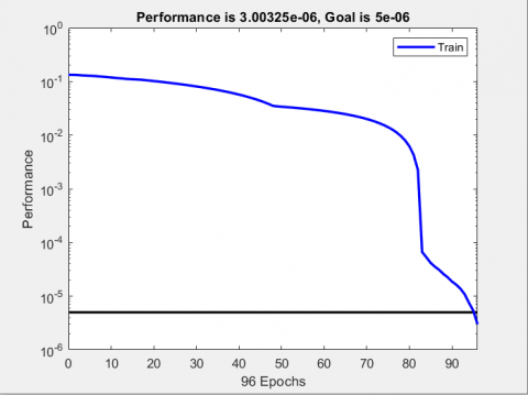
Figure 3. Training performance of the Diagnosis RBFNN
Figure 4. Training performance of the prognosis RBFNN
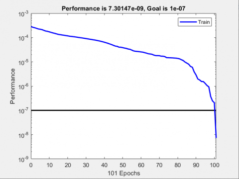
Figure 5. Training performance of the Remaining time RBFNN
Figures 3-5 represent the performances plots of the RBFNNs used respectively for diagnosis, prognosis, and the remaining time before a fault, these figures show how the MSE is minimized during the optimization of the RBFNNs without any indications and signs of the models under-fitting or over-fitting. We can clearly observe that the best values of MSE occur in the last 96 epochs of the learning cycle, with an associated MSE of approximately 3x10⁻⁶ for the RBFNN devoted to the diagnosis, 74 epochs, with MSE of 3.55x10⁻⁶, for the RBFNN dedicated to prognosis and 101 epochs, with MSE of 7,3x10⁻⁷ for the RBFNN associated to the remaining time before a fault, it is obvious that the values of MSEs are very close to the target MSE values, which indicate that the training targets are perfectly estimated. After the training operation, the RBFNNs are tested to a data composed of almost 70 temporal pairs. In order to measure the performances of the RBFNNs on the tested data, we are going to use the linear regression (R-value) plots, which measure the correlation between the targets and the RBFNNs outputs, so that the more the R-value is close to 1 the more the created model predictive abilities are excellent. The results of the testing process are represented respectively in Figures 6-8.
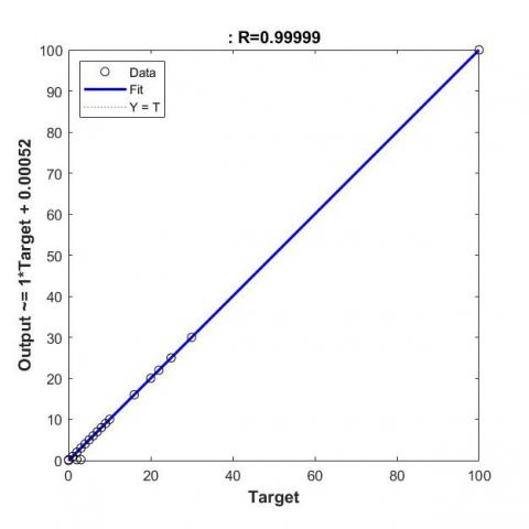
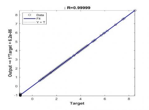
According to this figure, we can clearly observe that the values of regression are very close to 1(more than 0.999), i.e., practically all the data points (Circles) fall on the line of 45°, which indicate that the RBFNNs dispose on a great predictive ability, and can deal perfectly with the desired operations. After the building of the appropriate RBFNNs, we launch the trolly in order to transfer the product ‘A’, ‘B’, and ‘C’ and we create on purpose a faulty event in order to visualize in practice the response of the prognoses, the computer of the remaining time before a fault and the diagnostician. The results obtained are shown respectively in the Figures 9-17.
Figure 6. Testing performance of the Diagnosis RBFNN
Figure 7. Testing performance of the prognosis RBFNN
Figure 8. Testing performance of the remaining time RBFNN
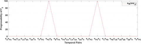
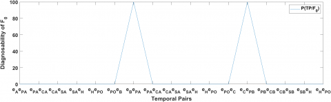
Figure 9. Prognosability of F0
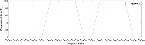
Figure 10. Prognosability of F1
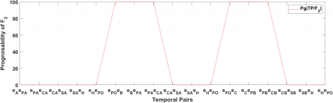
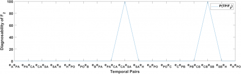
Figure 11. Prognosability of F2
Figure 12. Prognosability of F3
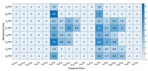
According to these results, it is clear that the diagnosticians have accurately detected the occurrence of the faulty events F0 (In the temporal pairs $e_{B}$ $e_{P A}$ and $e_{C}$ $e_{P B}$), $F_{1}$ (In the temporal pairs $e_{P A}$ $e_{C A}$, $e_{S A}$ $e_{H}$, $e_{P B}$ $e_{C B}$ and $e_{S B}$ $e_{H}$ ) and $F_{2}$ (In the temporal pairs $e_{C A}$ $e_{S A}$, $e_{C B}$ $e_{S B}$ ), by generating an occurrence probability of 100%, and which are already predicted by the prognosticator in the previous temporal pairs i.e. even before their occurance. The same thing for the faulty event F3, just in this case the probabilities are very law, which indicate that the occurrence of this fauty event is inexpectant. Moreover, thanks to the RBFNN dedicated to the calculation of the remaining time, it gave us an estimation of the interval of time when the faulty events can show up.
Figure 13. Remaining time before a fault result
Figure 14. Dignosability of F0
Figure 15. Diagnosability of F1
Figure 16. Diagnosability of F2
Figure 17. Diagnosability of F3
The discrete event system fault’s diagnosis and prognosis is a topic intensive and open of research so that it has been the subject of several researches and studies for many years. In these papers, we presented the theoretical framework to build an intelligent diagnostician and prognosticator based on feed-forward neural network, which allows the analysis of the large data extracted from the DES’s statistical model to deal with online diagnosis and prognosis. For this purpose, we proposed three feed-forward neural networks, which guarantee the computation of three main indexes: Diagnosability, Prognosability, and the Remaining time before a fault in such a way that determine the probably current and future state of the discrete event system as well as the interval of time, where a faulty event can probably occur in the coming functioning steps. As extension of this research, we are going to cover the second method, which is the DES diagnosis and prognosis using recurrent neural networks as well as the application of the approaches developed to a concrete industrial system to extract the results empirically.
This research was financially supported by the National Center for Scientific and Technical Research of Morocco. The authors wish to give their sincere thanks to this organism as well as we would like to thank the editors and reviewers for their constructive comments and suggestions, which helped us to improve the quality of these papers.
[1] Chan, F.T.S., Lau, H.C.W., Ip, R.W.L., Chan, H.K., Kong, S. (2005). Implementation of total productive maintenance: A case study. International Journal of Production Economics, 95(1): 71-94. https://doi.org/10.1016/j.ijpe.2003.10.021
[2] https://www.flexio.fr/maintenance-usine-4-0, accessed on 2 September 2021.
[3] Msaaf, M., Belmajdoub, F. (2015). L'application des réseaux de neurone de type «feedforward» dans le diagnostic statique. In Xème Conférence Internationale: Conception et Production Intégrées. https://hal.archives-ouvertes.fr/hal-01260830.
[4] Sampath, M., Sengupta, R., Lafortune, S., Sinnamohideen, K., Teneketzis, D. (1995). Diagnosability of discrete-event systems. IEEE Transactions on Automatic Control, 40(9): 1555-1575. https://doi.org/10.1109/9.412626
[5] Lunze, J., Schröder, J. (2001). State observation and diagnosis of discrete-event systems described by stochastic automata. Discrete Event Dynamic Systems, 11(4): 319-369. https://doi.org/10.1023/A:1011273108731
[6] Ammour, R. (2017). Contribution au diagnostic et pronostic des systèmes à évènements discrets temporisés par réseaux de Petri stochastiques (Doctoral dissertation, Normandie Université). https://tel.archives-ouvertes.fr/tel-01720312.
[7] Cabral, F.G., Moreira, M.V., Diene, O., Basilio, J.C. (2014). A Petri net diagnoser for discrete event systems modeled by finite state automata. IEEE Transactions on Automatic Control, 60(1): 59-71. https://doi.org/10.1109/TAC.2014.2332238
[8] Chen, J., Kumar, R. (2014). Stochastic failure prognosability of discrete event systems. IEEE Transactions on Automatic Control, 60(6): 1570-1581. https://doi.org/10.1109/TAC.2014.2381437
[9] Liu, B., Ghazel, M., Toguyéni, A. (2015). Model-based diagnosis of multi-track level crossing plants. IEEE Transactions on Intelligent Transportation Systems, 17(2): 546-556. https://doi.org/10.1109/TITS.2015.2478910
[10] Wang, H., Chen, P. (2011). Intelligent diagnosis method for rolling element bearing faults using possibility theory and neural network. Computers & Industrial Engineering, 60(4): 511-518. https://doi.org/10.1016/j.cie.2010.12.004
[11] Racoceanu, D. (2006). Contribution à la surveillance des Systèmes de Production en utilisant les Techniques de l’Intelligence Artificielle. Habilitation à diriger des recherches, Université de FRANCHE COMTÉ de Besançon, France. https://tel.archives-ouvertes.fr/tel-00011708.
[12] Tayarani-Bathaie, S.S., Vanini, Z.S., Khorasani, K. (2014). Dynamic neural network-based fault diagnosis of gas turbine engines. Neurocomputing, 125: 153-165. https://doi.org/10.1016/j.neucom.2012.06.050
[13] Xu, Y., Chen, Y.J., Zhu, Q.X. (2014). An extension sample classification‐based extreme learning machine ensemble method for process fault diagnosis. Chemical Engineering & Technology, 37(6): 911-918. https://doi.org/10.1002/ceat.201300622
[14] Cassandras, C.G., Lafortune, S. (2008). Introduction to Discrete Event Systems (Vol. 2). New York: Springer.
[15] Silva, M. (2018). On the history of discrete event systems. Annual Reviews in Control, 45: 213-222. https://doi.org/10.1016/j.arcontrol.2018.03.004
[16] Msaaf, M., Belmajdoub, F. (2018). Fault diagnosis and prognosis in discrete event systems using statistical model and neural networks. International Journal of Mechatronics and Automation, 6(4): 173-182. https://dx.doi.org/10.1504/IJMA.2018.095517
[17] Alur, R., Henzinger, T.A. (1992). Back to the future: towards a theory of timed regular languages. FOCS, 92: 177-186. https://doi.org/10.1109/SFCS.1992.267774
[18] Bouyer, P., Chevalier, F., D’Souza, D. (2005). Fault diagnosis using timed automata. International Conference on Foundations of Software Science and Computation Structures, Edinburgh, United Kingdom, pp. 219-233. https://doi.org/10.1007/978-3-540-31982-5_14
[19] Cassez, F., Grastien, A. (2013). Predictability of event occurrences in timed systems. International Conference on Formal Modeling and Analysis of Timed Systems, Buenos Aires, Argentina, pp. 62-76. https://doi.org/10.1007/978-3-642-40229-6_5
[20] Sayed-Mouchaweh, M. (2014). Discrete Event Systems: Diagnosis and Diagnosability. Springer Science & Business Media.
[21] Vignolles, A., Chanthery, E., Ribot, P. (2020). An overview on diagnosability and prognosability for system monitoring. European Conference of the Prognostics and Health Management Society (PHM Europe). https://hal.laas.fr/hal-02891028v2.
[22] Zaytoon, J., Lafortune, S. (2013). Overview of fault diagnosis methods for discrete event systems. Annual Reviews in Control, 37(2): 308-320. https://doi.org/10.1016/j.arcontrol.2013.09.009
[23] Sharkawy, A.N. (2020). Principle of neural network and its main types. Journal of Advances in Applied & Computational Mathematics, 7: 8-19.
[24] Haykin, S. (2010). Neural networks and learning machines, 3/E. Pearson Education India.
[25] Chollet, F. (2017). Deep Learning with Python, 1st edition. Shelter Island, New York: Manning Publications, 2017.
[26] Waibel, A., Hanazawa, T., Hinton, G., Shikano, K., Lang, K.J. (1989). Phoneme recognition using time-delay neural networks. IEEE Transactions on Acoustics, Speech, and Signal Processing, 37(3): 328-339. https://doi.org/10.1109/29.21701
[27] Sejnowski, T.J., Rosenberg, C.R. (1987). NETtalk: A parallel network that learns to read aloud. Complex Syst.,1: 145-168.
[28] Faris, H., Aljarah, I., Mirjalili, S. (2017). Evolving radial basis function networks using moth–flame optimizer. Handbook of Neural Computation, pp. 537-550.
[29] Zemouri, R. (2003). Contribution à la surveillance des systèmes de production à l'aide des réseaux de neurones dynamiques: Application à la e-maintenance (Doctoral dissertation, Université de Franche-Comté).
[30] Patan, K. (2008). Artificial Neural Networks for The Modelling and Fault Diagnosis of Technical Processes. Springer.
[31] Moody, J., Darken, C.J. (1989). Fast learning in networks of locally-tuned processing units. Neural Computation, 1(2): 281-294. https://doi.org/10.1162/neco.1989.1.2.281
[32] Broomhead, D.S., Lowe, D. (1988). Radial basis functions, multi-variable functional interpolation and adaptive networks. Royal Signals and Radar Establishment Malvern (United Kingdom).
[33] https://machinelearningmastery.com/how-to-prepare-categorical-data-for-deep-learning-in-python, accessed on 2 September 2021.
[34] Kopal, I., Harničárová, M., Valíček, J., Krmela, J., Lukáč, O. (2019). Radial basis function neural network-based modeling of the dynamic thermo-mechanical response and damping behavior of thermoplastic elastomer systems. Polymers, 11(6): 1074. https://doi.org/10.3390/polym11061074