Bouiri Abdesselam* | Benoudjafer Cherif | Boughazi Othmane
© 2021 IIETA. This article is published by IIETA and is licensed under the CC BY 4.0 license (http://creativecommons.org/licenses/by/4.0/).
OPEN ACCESS
In order to control output powers generated by doubly fed induction generator (DFIG) used in wind application (WA) many previous studies, mainly based on flux orientation control (FOC) and neglecting resistance to get a simple model of DFIG with decoupled axis. However, this control strategy requires several hypotheses: low and stability of grid voltage in order to orientated the statoric flux, high power of generator to neglecting statoric resistance. As a result that may not be present in realty due to direct connection between stator and the grid In addition to the presence of resistance, whatever the power of the generator, therefore the DFIG represents a complex model and required a nonlinear control without previous approaches closer to reality to respond highly against DFIG nonlinear model, this is the first paper presents a novel strategy to control nonlinear model of DFIG based on substitution method to solving (d,q) coupled axes without flux orientation and neglecting resistance (FOANR) and also does not take into account stability of grid voltage, for produce required reference active and reactive power by controlling the voltage of rotor side converter (RSC), using classical proportional-integral (PI) controller in a non-linear synthesis form by three methods :direct control (D) and indirect open loop (IOL) and indirect with power loop (IWPL),we compared three controls and check their performance towards the real model of DFIG to verify our control and proving its effectiveness without previous approaches. Finally, the simulation results of the studied controls are presented, analyzed and compared.in terms of power reference tracking, robustness to the parametric variation and the ability to respond to sudden wind speed variation.
wind application (WA), doubly fed induction generator (DFIG), nonlinear model, flux orientation and neglecting resistance (FOANR), proportional-integral (PI)
The use of wind energy has become a must in addition to solar energy as alternative energy, free and clean than fossil energy for this reason many studies focus on controlling techniques in proportion to the requirements of effectiveness and cost.
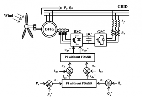
That is why today in field of wind energy many manufacture like Gamesa and Alstom-Ecotecnia [1]. developed wind turbine based on doubly fed induction generator to answer on the specifications related to effectiveness against fixe wind speed and high-cost converters, that is the main defect in previous design generators like a squirrel cage induction generator (SCIG) requires must worked only at fixe speed wind with a mechanical control system, these disadvantages are solved and improved when connect the wind turbine by permanent magnet synchronous generator (PMSG) [2], this last type used to create electrical control completely decoupled from the mechanical system and become working on a variable wind speed, however in this solution remained the high cost defect of converters in order to supply generated powers into grid,, the doubly fed induction generator (DFIG) is the optimal solution response to variable wind speed +30% and -30% from the normal speed of the generator with a low cost of converter as well as many other advantage we mention of them return loss rotor power to the grid at high wind speed Figure 1 and reduce the control of the mechanical system. thanks to the wide range variation of the wind speed.
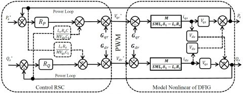
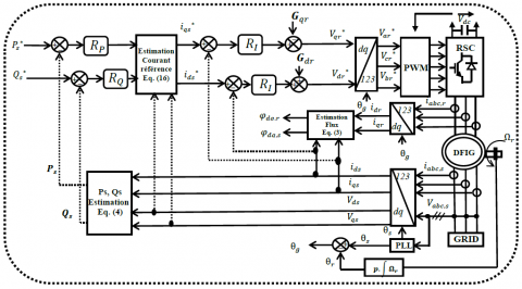
Figure 1. Configuration of wind application based on DFIG using PI-IWPL controller without FOANR
In recent years, studies related to control powers of DFIG using a simplified model of the latter by flux orientation and neglecting the statoric resistance. The filed oriented control (FOC) strategy is the most popular control [3-5]. providing a complete decoupled between rotor and stator similar to DC motor, Through FOC combined with neglecting the statoric resistance leads to control the DFIG using linear controller like proportional-integral PI [6-8]. So, the control powers of DFIG can only through vector control of flux or voltage grid [9]. However, these approaches just apply for a simple model which does not take into account the stator resistance because sometimes the modeling under hypothesis of considered a generator is of high power produce more than 1 MW, hence we can say no matter how high power of the generator, actually its resistance not neglected, there is study based on non-neglected stator resistance [10]. But it is based on flux orientation by supposing that the electrical supply network is stable, on the other hand, what is the strategy about the DFIG real model connected to the grid and has actual value of statoric flux in quadratic axis? In this case the control used it is less efficient and performance due to the non-linear model expressed by multivariable equation with value of flux in both axes (d,q) as results it will give us non-reliable results in the reality because of the existence of those approaches.
This prompted us to develop a new strategy of control applicable on the nonlinear model of the doubly fed induction generator based on substitution method without flux orientation control and also without neglected stator resistance and unlike previous studies we take all function nonlinear of DFIG for linear regulator proportional integrator (PI), to control of power energy from the rotor side converter (RSC) with a Pulse Width Modulation (PWM), the PI control is developed by three methods: The most popular direct method PI-(D) and indirect method open loop (IOL) and finally for high performance and efficient we apply PI indirect with power loop method (IWPL), the purpose of analysis and comparison among these methods is to show the control synthesis for each method and any one more responsive to the complete model of DFIG, their performances are evaluated and compared in terms of power reference tracking, robustness with respect to sudden changes in speed and robustness with respect to parameters variation.
This paper presents firstly a nonlinear DFIG model based on nonlinear equation of DFG without any precious approaches based on substitution method and then we apply PI controller by three methods to control directly stator current without resorting to control the rotor current as in previous studies based on flux orientation and neglecting stator resistance, Finally, we get three methods of nonlinear control that we compared it to demonstrate the performance and effectiveness of our control over any variables and changing of DFIG nonlinear model After confirming the effectiveness of the three controllers that we developed, we compare the performance of the most effective method, which is indirect with power loop (IWPL) based on substitution method we call it full control (FC) compared o with same method but based FOC and neglecting resistance and we call it simple control (SC) This is in order to know the simple control defect and the addition presented by this paper to control the non-linear model of the DFIG using in wind application.
The coupled model of DFIG can described through equivalent circuit Figure 2 in park (d, q) reference frame, and we can write the expressions of stator, rotor voltages and flux components It can be written in terms of stator and rotor resistance for the voltage and stator, rotor flux in terms of statoric and rotoric inductances as follows [11-14].
Figure 2. Equivalent circuit of DFIG in park reference frame
$\left\{ \begin{align} & {{v}_{ds}}={{R}_{s}}{{i}_{ds}}+\frac{d{{\phi }_{ds}}}{dt}-{{w}_{s}}{{\phi }_{qs}} \\& {{v}_{qs}}={{R}_{s}}{{i}_{qs}}+\frac{d{{\phi }_{qs}}}{dt}+{{w}_{s}}{{\phi }_{ds}} \\ & {{v}_{dr}}={{R}_{r}}{{i}_{dr}}+\frac{d{{\phi }_{dr}}}{dt}-{{w}_{g}}{{\phi }_{qr}} \\ & {{v}_{qr}}={{R}_{r}}{{i}_{qr}}+\frac{d{{\phi }_{qr}}}{dt}+{{w}_{g}}{{\phi }_{dr}} \\\end{align} \right.$ (1)
ids, iqs, idr, iqr– two-phase statoric and rotoric currents,
${{w}_{g}}={{w}_{s}}-{{w}_{r}}$ (2)
Wg, Ws, Wr – synchronous and rotor angular speeds for rotor current and stator and Mechanical.
$\left\{ \begin{align} & {{\phi }_{ds}}={{L}_{s}}{{i}_{ds}}+M{{i}_{dr}} \\ & {{\phi }_{qs}}={{L}_{s}}{{i}_{qs}}+M{{i}_{qr}} \\& {{\phi }_{dr}}={{L}_{r}}{{i}_{dr}}+M{{i}_{ds}} \\ & {{\phi }_{qr}}={{L}_{r}}{{i}_{qr}}+M{{i}_{qs}} \\\end{align} \right.$ (3)
The stator active and reactive powers are written:
$\left\{ \begin{align} & {{p}_{s}}={{v}_{ds}}{{i}_{ds}}+{{v}_{qs}}{{i}_{qs}} \\ & {{Q}_{s}}={{v}_{qs}}{{i}_{ds}}-{{v}_{ds}}{{i}_{qs}} \\ \end{align} \right.$ (4)
2.1 Modeling of DFIG based on substitution method
By substituting the flux Eq. (3) in the stator and rotor voltage Eq. (1) we obtain:
$\left\{ \begin{align} & {{v}_{ds}}={{R}_{s}}{{i}_{ds}}+{{L}_{s}}\frac{d{{i}_{ds}}}{dt}+M\frac{d{{i}_{dr}}}{dt}-{{w}_{s}}{{\phi }_{qs}} \\ & {{v}_{qs}}={{R}_{s}}{{i}_{qs}}+{{L}_{s}}\frac{d{{i}_{qs}}}{dt}+M\frac{d{{i}_{qr}}}{dt}+{{w}_{s}}{{\phi }_{ds}} \\& {{v}_{dr}}={{R}_{r}}{{i}_{dr}}+{{L}_{r}}\frac{d{{i}_{dr}}}{dt}+M\frac{d{{i}_{ds}}}{dt}-{{w}_{g}}{{\phi }_{qr}} \\ & {{v}_{qr}}={{R}_{r}}{{i}_{qr}}+{{L}_{r}}\frac{d{{i}_{qr}}}{dt}+M\frac{d{{i}_{qs}}}{dt}+{{w}_{g}}{{\phi }_{dr}} \\\end{align} \right.$ (5)
By using the equation system (5), we can establish the expression of the rotor current variation in the stator:
$\left\{ \begin{align} & \overset{\bullet }{\mathop{{{i}_{dr}}}}\,=\frac{1}{M}\left[ {{v}_{ds}}-{{R}_{s}}{{i}_{ds}}-{{L}_{s}}{{\overset{\bullet }{\mathop{i}}\,}_{ds}}+{{w}_{s}}{{\phi }_{qs}} \right] \\ & \overset{\bullet }{\mathop{{{i}_{qr}}}}\,=\frac{1}{M}\left[ {{v}_{qs}}-{{R}_{s}}{{i}_{qs}}-{{L}_{s}}{{\overset{\bullet }{\mathop{i}}\,}_{qs}}-{{w}_{s}}{{\phi }_{ds}} \right] \\\end{align} \right.$ (6)
Also, using the Eq. (5) we can establish the expression of the rotor current variation in the rotor:
$\left\{ \begin{align} & \overset{\bullet }{\mathop{{{i}_{dr}}}}\,=\frac{1}{{{L}_{r}}}\left[ {{v}_{dr}}-{{R}_{r}}{{i}_{dr}}-M{{\overset{\bullet }{\mathop{i}}\,}_{ds}}+{{w}_{g}}{{\phi }_{qr}} \right] \\ & \overset{\bullet }{\mathop{{{i}_{qr}}}}\,=\frac{1}{{{L}_{r}}}\left[ {{v}_{qr}}-{{R}_{r}}{{i}_{qr}}-M{{\overset{\bullet }{\mathop{i}}\,}_{qs}}-{{w}_{g}}{{\phi }_{dr}} \right] \\\end{align} \right.$ (7)
By substituting (6) in (7), the variation of the rotor current in the stator and in the rotor, we can establish the variation of the stator current by this relation which directly connects with the rotor voltages:
$\left\{ \begin{align} & \overset{\bullet }{\mathop{{{i}_{ds}}}}\,=\frac{1}{{{L}_{r}}{{\delta }_{1}}}{{v}_{dr}}+\frac{1}{{{L}_{r}}{{\delta }_{1}}}\left( {{w}_{g}}{{\phi }_{qr}}-{{R}_{r}}{{i}_{dr}} \right)+\frac{1}{M{{\delta }_{1}}}\left( {{R}_{s}}{{i}_{ds}}-{{v}_{ds}}-{{w}_{s}}{{\phi }_{qs}} \right) \\ & \overset{\bullet }{\mathop{{{i}_{qs}}}}\,=\frac{1}{{{L}_{r}}{{\delta }_{1}}}{{v}_{qr}}-\frac{1}{{{L}_{r}}{{\delta }_{1}}}\left( {{w}_{g}}{{\phi }_{dr}}+{{R}_{r}}{{i}_{qr}} \right)+\frac{1}{M{{\delta }_{1}}}\left( {{R}_{s}}{{i}_{qs}}-{{v}_{qs}}+{{w}_{s}}{{\phi }_{ds}} \right) \\\end{align} \right.$ (8)
${{\delta }_{1}}=\frac{M}{{{L}_{r}}}-\frac{{{L}_{s}}}{M}$ (9)
We applied the place transformation on the equation (8) we get as follows:
$\left\{ \begin{align} & {{v}_{qr}}=\left[ \frac{M{{L}_{r}}{{\delta }_{1}}S-{{L}_{r}}{{R}_{s}}}{M} \right]{{i}_{qs}}+\left( {{w}_{g}}{{\phi }_{dr}}+{{R}_{r}}{{i}_{qr}} \right)-\frac{{{L}_{r}}}{M}\left( {{w}_{s}}{{\phi }_{ds}}-{{v}_{qs}} \right) \\ & {{v}_{dr}}=\left[ \frac{M{{L}_{r}}{{\delta }_{1}}S-{{L}_{r}}{{R}_{s}}}{M} \right]{{i}_{ds}}-\left( {{w}_{g}}{{\phi }_{qr}}-{{R}_{r}}{{i}_{dr}} \right)+\frac{{{L}_{r}}}{M}\left( {{w}_{s}}{{\phi }_{qs}}+{{v}_{ds}} \right) \\\end{align} \right.$ (10)
where, S is the Laplace operator.
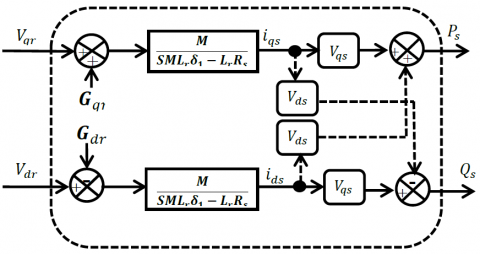
Figure 3. Nonlinear model of DFIG without FOANR
After we were able to achieve the real model of DFIG Eq. (10) without resorting to vector control by flux orientation and neglecting the statoric resistance, by means of a first order transfer function (Figure 3) that directly links the rotor voltage with the statoric current, we will move to find the relationship between the statoric current and the power of DFIG, for the final synthesis of the control.
From the nonlinear model (Eq. (4)), the expression of the active and reactive stator powers (Eq. (11)) presenting a nonlinear model, with a coupling between the control variables, ids, iqs, this non-linearity can be treated by a unification of the axes for each power.
$\left\{ \begin{align} & {{p}_{s}}={{v}_{ds}}{{i}_{ds}}+{{v}_{qs}}{{i}_{qs}}\Rightarrow {{\overset{\bullet }{\mathop{p}}\,}_{s}}={{v}_{ds}}{{\overset{\bullet }{\mathop{i}}\,}_{ds}}+{{v}_{qs}}{{\overset{\bullet }{\mathop{i}}\,}_{qs}} \\ & {{Q}_{s}}={{v}_{qs}}{{i}_{ds}}-{{v}_{ds}}{{i}_{qs}}\Rightarrow {{\overset{\bullet }{\mathop{Q}}\,}_{s}}={{v}_{qs}}{{\overset{\bullet }{\mathop{i}}\,}_{ds}}-{{v}_{ds}}{{\overset{\bullet }{\mathop{i}}\,}_{qs}} \\\end{align} \right.$ (11)
The idea is based on the Mathematical transfer of non-linear writing at the level of stator currents towards powers to have a control of each power by each control quantity.
We can write stator currents in terms of active power:
$\left\{ \begin{align} & {{i}_{ds}}=\frac{1}{{{v}_{ds}}}\left[ {{p}_{s}}-{{v}_{qs}}{{i}_{qs}} \right] \\ & {{i}_{qs}}=\frac{1}{{{v}_{qs}}}\left[ {{p}_{s}}-{{v}_{ds}}{{i}_{ds}} \right] \\\end{align} \right.$ (12)
Also using Eq. (11) we determine the stator currents in terms of reactive power:
$\left\{ \begin{align} & {{i}_{ds}}=\frac{1}{{{v}_{qs}}}\left[ {{Q}_{s}}+{{v}_{ds}}{{i}_{qs}} \right] \\& {{i}_{qs}}=\frac{1}{{{v}_{ds}}}\left[ {{v}_{qs}}{{i}_{ds}}-{{Q}_{s}} \right] \\\end{align} \right.$ (13)
By substituting (13) in (12), and to control the active power along the q axis and the Reactive power along the d axis we obtain the expression which links the stator currents with the coupled powers: we can write:
$\left\{ \begin{align}& {{p}_{s}}={{v}_{ds}}{{c}_{1}}{{i}_{qs}}+c{{Q}_{s}} \\& {{Q}_{s}}={{v}_{qs}}c{{c}_{1}}{{i}_{ds}}-c{{p}_{s}} \\\end{align} \right.$ (14)
$c=\frac{{{v}_{ds}}}{{{v}_{qs}}}\text{et}$ ${{c}_{1}}=\frac{1}{c}+\text{c}$ (15)
From Eq. (14) we determine the reference currents from the reference powers:
$\left\{ \begin{align} & {{i}_{qs}}=\frac{1}{{{v}_{ds}}{{c}_{1}}}\left[ {{p}_{s}}-c{{Q}_{s}} \right]\Rightarrow \overset{*}{\mathop{{{i}_{qs}}}}\,=\frac{1}{{{v}_{ds}}{{c}_{1}}}\left[ \overset{*}{\mathop{{{p}_{s}}}}\,-c\overset{*}{\mathop{{{Q}_{s}}}}\, \right] \\ & {{i}_{ds}}=\frac{1}{{{v}_{qs}}{{c}_{1}}}\left[ {{p}_{s}}+\frac{1}{c}{{Q}_{s}} \right]\Rightarrow \overset{*}{\mathop{{{i}_{ds}}}}\,=\frac{1}{{{v}_{qs}}{{c}_{1}}}\left[ \overset{*}{\mathop{{{p}_{s}}}}\,+\frac{1}{c}{{\overset{*}{\mathop{Q}}\,}_{s}} \right] \\\end{align} \right.$ (16)
In this paper, we simply transfer the non-linear writing from the output to the input meaning from the grid current (direct and quadratic current) to the energy and thus it will be easy for us to control whatever the Active and Reactive powers value is variable and applied to the system because according to the definition of control is that the output follows ideally any input we want to apply to the system.
The PI controller without flux orientation and negligence statoric resistance to control active and reactive powers DFIG by three methods direct and indirect open loop and indirect method with power loop, from the Eqns. (10) and (16) we notice that the rotoric voltage connected with the current (indirect) and with the power (direct) by a first order transfer function.
4.1 Indirect open loop (IOL) synthesis method
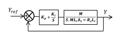
The indirect method open loop using PI controller (PI-IOL) to control real model of DFIG without flux orientation and negligence statoric resistance, it requires us to use the Eq. (10) directly: In our case, the transfer function corresponds to the current regulators (RI) is given by ( $\left(K_{p}+K_{i} / S\right)$ ) in Figure 5. The Open Loop Transfer Function (OLTF) in Figure 4 with the regulators is written as follows:
$OLTF=\frac{\left( S+\frac{{{K}_{i}}}{{{K}_{p}}} \right)}{\frac{S}{{{K}_{p}}}}\frac{\frac{M}{M{{L}_{r}}{{\delta }_{1}}}}{\left( S-\frac{{{R}_{s}}{{L}_{r}}}{M{{L}_{r}}{{\delta }_{1}}} \right)}$ (17)
We choose the pole compensation method [15-17] for the synthesis of the regulator in order to eliminate the zero of the transfer functions. This leads to the following equality.
$\frac{{{K}_{i}}}{{{K}_{p}}}=-\frac{{{R}_{s}}}{M{{\delta }_{1}}}$ (18)
The Open Loop Transfer Function is obtained:
$OLTF=\frac{{{K}_{p}}}{S{{L}_{r}}{{\delta }_{1}}}$ (19)
The closed loop transfer function for first order transfer function It is given as follows:
$CLTF=\frac{1}{1+\tau .S}$ (20)
τ Response time of the system which is fixed on the order of 10 ms.
The closed loop transfer function (CLTF) in (Eq. (20)) it can be written:
$CLTF=\frac{1}{1+\tau .S}=\frac{1}{1+\frac{1}{OLTF}}$ (21)
By identification we find that:
$\tau .S=\frac{1}{OLTF}=\frac{S{{L}_{r}}{{\delta }_{1}}}{{{K}_{p}}}$ (22)
By using the Eqns. (22) and (18) we can therefore express the gains of the correctors as a function of the machine parameters and the response time:
${{K}_{p}}=\frac{{{L}_{r}}{{\delta }_{1}}}{\tau }$, ${{K}_{i}}=\frac{-{{L}_{r}}{{R}_{s}}}{M.\tau }$ (23)
We put in equation Eq. (10) as shown in Figure 5:
$\left\{ \begin{align} & {{G}_{qr}}=\frac{{{L}_{r}}}{M}({{w}_{s}}{{\phi }_{ds}}-{{V}_{qs}})-({{R}_{r}}{{i}_{qr}}+{{w}_{g}}{{\phi }_{dr}}) \\ & {{G}_{dr}}=\frac{{{L}_{r}}}{M}({{w}_{s}}{{\phi }_{qs}}+{{V}_{ds}})+({{R}_{r}}{{i}_{dr}}-{{w}_{g}}{{\phi }_{qr}}) \\\end{align} \right.$ (24)
Figure 4. System regulated by PI controller
Figure 5. Indirect open loop method (IOL) using PI without FOANR for DFIG nonlinear model
4.2 Direct (D) synthesis method
By substituting the Eq. (16) in the Eq. (10), to have a direct control of the powers, where the voltages are linked to the powers by a transfer function of the first order:
$\left\{ \begin{align}& {{v}_{qr}}=\left( \frac{M{{L}_{r}}{{\delta }_{1}}S-{{L}_{r}}{{R}_{s}}}{M{{V}_{ds}}{{c}_{1}}} \right){{P}_{S}}+\frac{{{L}_{r}}{{R}_{s}}c}{M{{V}_{ds}}{{c}_{1}}}{{Q}_{s}}+{{G}_{qr}} \\ & {{v}_{dr}}=\left( \frac{M{{L}_{r}}{{\delta }_{1}}S-{{L}_{r}}{{R}_{s}}}{M{{V}_{qs}}c{{c}_{1}}} \right){{Q}_{S}}-\frac{{{L}_{r}}{{R}_{s}}}{M{{V}_{qs}}{{c}_{1}}}{{P}_{s}}+{{G}_{dr}} \\\end{align} \right.$ (25)
In this case, we notice that the voltage is connected with two Transfer functions, the transfer function (Kp1+Ki1/S) corresponds to RP and (Kp2+Ki2/S) corresponds to the RQ regulators in Figure 6, and by same previous way we can express the gains of the correctors.
$\left\{ \begin{align} & {{K}_{p1}}=\frac{{{L}_{r}}{{\delta }_{1}}}{{{\tau }_{1}}.{{V}_{ds}}{{c}_{1}}},{{K}_{i1}}=-\frac{{{R}_{s}}{{L}_{r}}}{{{\tau }_{1}}.M.{{V}_{ds}}{{c}_{1}}} \\& {{K}_{p2}}=\frac{{{L}_{r}}{{\delta }_{1}}}{{{\tau }_{1}}.{{V}_{qs}}c{{c}_{1}}},{{K}_{i2}}=-\frac{{{R}_{s}}{{L}_{r}}}{{{\tau }_{1}}.M.{{V}_{qs}}c{{c}_{1}}} \\\end{align} \right.$ (26)
Figure 6. Direct method (D) using PI without FOANR for DFIG nonlinear model
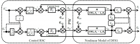
4.3 Indirect with power loop (IWPL) synthesis method
This control method is among the preferred strategies of control because it is highly efficient and is a result of the previous methods it uses two controllers of previous methods (direct and indirect) on each axis for robustness and highly efficient control. With only one note which is: to calculate the coefficients of the controllers kp and ki in each axis, The response time τ correspond to RP regulators, RQ must be less than the response time τ1 corresponds to RI regulators: τ1<τ.
Figure 7. Configuration of indirect method with power loop (IWPL) using PI without FOANR for DFIG nonlinear model
The three methods PI-(D) and PI-(IOL) and PI-(IWPL) are simulated and compared regarding reference active and reactive power produced by real model of DFIG using a PI type controller.
5.1 Tracking test
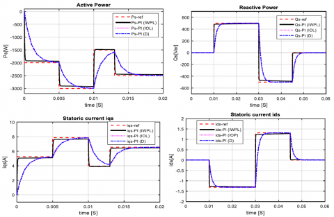
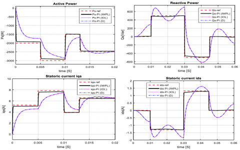
In this test, we compare the performance of each method under a nominal speed of the generator without external (wind speed variation) or internal perturbation (parametric variation), by changing the reference power produced Figure 8 show the response of active and reactive power of DFIG by the PI-D and PI-IOL PI-IWPL controller, with also considering the and statoric currents at different time periods to ensure the ability of each controller to maintain the required reference.
5.2 Robustness tests
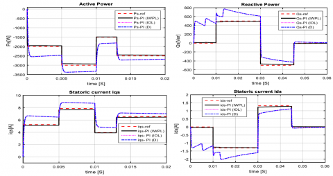
In this test the generator has an internal perturbation due to parametric variation of DFIG under saturation of magnetic circuit M+5% and an increasing in temperature which leads to an increasing in resistance Rr, Rs+50% through the results shown in Figures 9, 10, it is possible to know the robust of each response controller for this disturbance.
Figure 8. Power and current response (reference tracking test)
Figure 9. Power and current response with parametric variations (M+5%)
Figure 10. Power and current response with parametric variations (Rr, Rs+50%)
5.3 Sensitivity to perturbations
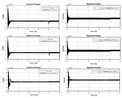
In this test we check that the controllers are able to respond to a change in wind speed Wr+60% at 4s with PWM, to know the extent of its response to wind speed variation to maintain the required reference (Pref=-5000 w supply of power to the network and Qref=0Var keep a unit power factor cosφ=1 grid side) of power as well as the power qualities in the presence of the rotor side converter (Figure 11).
After comparing the three Method with new strategy, we worked to verify the effectiveness of the strategy based on Substitution Method with the classical method based on Flux orientation (FOC) and neglecting stator resistance.
Figure 11. Active and reactive power response to a speed variation
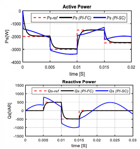
Since the substitution strategy takes the nonlinear synthesis, we called it full control (FC) and since the Flux oriented control (FOC) is directed only to control the simple model of the DFIG we called it simple control (SC). However, both control method (FC-SC) in this paper directed for controlling the complete model of DFIG We have chosen the best method through the previous results to compare FC and SC, which is the direct control with power loop.
We can know the behavior of the controllers through simulation results (Figure 12) without any perturbation under fixe speed generator and without changes in its parameters; the control powers of DFIG real model during high response: showed that PI full controller (PI-FC), is more efficient than the control using simple controller (SC-PI) which is far from the reference point, hence is not responding quickly.
Figure 12. Powers response (reference tracking test)
We can verify the effectiveness of the two control methods by robustness Tests, with the rise value of the resistance, (w(Rr, RS)+50% which makes a big difference in the assumption of the simple control because it does not have an input of statoric resistance compared to the full controller The control powers generated by the DFIG real model without FONR are shown in results Figure 13, that the controllers, Rr, Rs+50%) a rise in temperature, this effect is very high and clear for the simple controller PI-SC especially under a rise in resistances ,It has a low response away from the required reference point unlike the full controller PI-FC showed robustness in the control, by staying at the nearest reference point during changing the parameters.
Figure 13. Power response under a rise in temperature (Rr, Rs+50%)
After this paper, and through the results shown in the (Figures 8/9), we can say that we have demonstrated the ability of the substitution method to control the complete of DFIG without FOC and neglecting the resistance.
This article deals the control of the powers generated from a wind power system based-on doubly fed induction generation for the first time based on substitution method without resorting to FOC and neglecting the stator resistance using nonlinear synthesis control with proportional-integral controller (PI) by three control methods, its effectiveness has proven towards the nonlinear model of DFIG.
Where the nonlinear write transferred from the control stator currents (Eq. (4)) to the reference power and to the measured powers: in the indirect (Figure 5) and direct methods (Figure 6) respectively without decoupled between (d,q) axes as in simple control.
Through the simulation results, the nonlinear synthesis by three methods using PI controller applied to real model of DFIG to control active and reactive power by controlling current stator directly to adjust the reference value of the rotor voltage regarding reference tracking tests without any perturbation (Figure 8), the three methods showed an acceptable result and provide a good performance against the coupled model of DFIG.
Direct PI (D) and indirect open loop control PI(IOL) gives the same results due both has same synthesis of control with same response time that is why their results (The curve is applied to the other),however the indirect with power loop control PI (IWPL) show more effective than previous methods because it has two processing and doubly control loops ,loop for control the power and loop to control the current (Figure 7) so we find it robust (Figure 9) when a change in the DFIG parameters the IWPL method remained a certain fixed percentage of error opposite than the direct and indirect method which showed move away from the reference value with a greater value especially for variation resistance (Rr Rs +50%) in the reactive power control.
Regarding sensitivity to perturbations against sudden wind speed variation, the direct and indirect methods respond to this sudden change responded by a peak which produces at the time of speed variation and disappears at the same second with a high error rate than before, an indication of power loss as for the indirect PI (IWPL) control response this peak does not appear at all, an indication that it is robust and less affected by the change in wind speed.
The DFIG parameters:
Pn= 7.5 KW, Vs= 220/380 V, fs = 50 Hz, P = 2, Ω =1430 tr/min, Rs = 0.455 Ω, Rr = 0.62 Ω, Ls = 0.084 H, Lr = 0.081 H, M = 0.078 H, f = 0.00673 N.s/rad, J = 0.3125 kg.m2.
[1] Abad, G., Lopez, J., Rodriguez, M., Marroyo, L., Iwanski, G. (2011). Doubly Fed Induction Machine: Modeling and Control for Wind Energy Generation. John Wiley & Sons, 85: 74-76.
[2] Rekioua, D. (2014). Wind Power Electric Systems Modeling, Simulation and Control. Springer-Verlag London. 15-20. https://doi.org/10.1007/978-1-4471-6425-8
[3] Pena, R., Clare, J.C., Asher, G.M. (1996). A doubly fed induction generator using back-to-back PWM converters supplying an isolated load from a variable speed wind turbine. IEE Proceedings-Electric Power Applications, 143(5): 380-387. http://dx.doi.org/10.1049/ip-epa:19960454
[4] Atkinson, D.J., Lakin, R.A., Jones, R. (1997). A vector-controlled doubly-fed induction generator for a variable-speed wind turbine application. Transactions of the Institute of Measurement and Control, 19(1): 2-12. https://doi.org/10.1177/014233129701900101
[5] Muller, S., Deicke, M., De Doncker, R.W. (2002). Doubly fed induction generator systems for wind turbines. IEEE Industry applications magazine, 8(3): 26-33. https://doi.org/10.1109/2943.999610
[6] Mohamed, M.B., Jemli, M., Gossa, M., Jemli, K. (2004). Doubly fed induction generator (DFIG) in wind turbine modeling and power flow control. In 2004 IEEE International Conference on Industrial Technology, 2: 580-584. https://doi.org/10.1109/ICIT.2004.1490139
[7] Pena, R.S., Clare, J.C., Asher, G.M. (1996). Vector control of a variable speed doubly-fed induction machine for wind generation systems. EPE Journal, 6(3-4): 60-67. https://doi.org/10.1080/09398368.1996.11463397
[8] Ouamri, B., Ahmed, Z.F. (2018). Comparative analysis of robust controller based on classical proportional-approach for power control of wind energy system. Rev. Roum. Sci. Techn.-Électrotechn.et Énerg, 63(2): 210-216.
[9] Hu, J.B., He, Y.K., Zhu, J.G. (2006). The internal model current control for wind turbine driven doubly-fed induction generator. In Conference Record of the 2006 IEEE Industry Applications Conference Forty-First IAS Annual Meeting, 1: 209-215. https://doi.org/10.1109/IAS.2006.256525
[10] Boudjema, Z., Meroufel, A., Djerriri, Y. (2013). Nonlinear control of a doubly fed induction generator for wind energy conversion. Carpathian Journal of Electronic & Computer Engineering, 6(1): 28-35.
[11] Hofmann, W., Okafor, F. (2001). Optimal control of doubly-fed full-controlled induction wind generator with high efficiency. In IECON'01. 27th Annual Conference of the IEEE Industrial Electronics Society (Cat. No. 37243), 2: 1213-1218. https://doi.org/10.1109/IECON.2001.975955
[12] Caron, J.P., Hautier, J.P. (1995). Electrotechnique Modélisation et commande de la machine asynchrone. Presses Universitaires de Strasbourg, pp. 53-57.
[13] Abad, G., López, J., Rodríguez, M., Marroyo, L., Iwanski, G. (2011). Doubly Fed Induction Machine: Modeling and Control for Wind Energy Generation Applications. Wiley-IEEE Press, 139-143.
[14] Fayssal, A., Chaiba, A., Babes, B., Mekhilef, S. (2016). Design and implementation of high performance field oriented control for grid-connected doubly fed induction generation via hysteresis rotor current controller. Revue Roumaine des Sciences Techniques - Serie Électrotechnique et Énergétique, 61(4): 319-324.
[15] Boyette, A., Saadate, S., Poure, P. (2006). Direct and indirect control of a Doubly Fed Induction Generator wind turbine including a storage unit. IECON 2006 - 32nd Annual Conference on IEEE Industrial Electronics, pp. 2517-2522. https://doi.org/10.1109/IECON.2006.347300
[16] Kerrouchea, K., Mezouarb, A., Belgacema, K. (2013). Decoupled control of doubly fed induction generator by vector control for wind energy conversion system. Elsevier Energy Procedia, 42: 239-248. https://doi.org/10.1016/j.egypro.2013.11.024
[17] De Larminat, P. (1996). Automatique. Commande des Systèmes Linéaires, Seconde Edition, Paris, Hermès, 1996.