Farid Berrezzek* | Abdelhak Benheniche
© 2021 IIETA. This article is published by IIETA and is licensed under the CC BY 4.0 license (http://creativecommons.org/licenses/by/4.0/).
OPEN ACCESS
This work proposes a sensorless control strategy for the induction motor (IM) using a Backstepping control and a nonlinear observer based on the circle-criterion approach. The Backstepping is a powerful control strategy that deals with nonlinear higher-order systems and includes non-measurable parameters related to the (IM). The nonlinear observer approach is intended to determine these important parameters. The circle-criterion approach is employed to determine the observer gain matrices as a solution of LMI (linear matrix inequalities) that guarantee the stability conditions of the designed observer. The main objective of this method is to solve the problem of the nonlinearities of the system which ensure the global asymptotic convergence of the observed dynamics and to improve the performance of the induction motors. The efficiency and correctness of the proposed scheme are proven by several numerical simulations.
induction motor, nonlinear control, backstepping control, nonlinear observer, circle criterion, Lyapunov stability
The induction motors are the most useful motors in electrical modern industrial society, because of their good performance: simplicity, robustness, low price and easy maintenance necessities [1, 2]. However, (IM) are known as multivariable nonlinear time-varying systems. Thus, entail other problems for motor control, fault diagnostic and conditions monitoring [1]. In the past years, and with technological advancements in power electronics and digital electronics field, several nonlinear control theories of the induction motor have been proposed and became industrial standard for medium and high performance applications. They were formulated and developed to replace classical control strategies such as scalar control and vector control which can ensure limited performance. In several industrial applications, it is indispensable to use more advanced controls which are consistent with the envisaged performance but more complex. Among the strategies applied to induction motor control that ensure high performance, we find, the input-output feedback linearization technique, the passivity-based control, the flatness strategy, the sliding mode technique and hybrid control [3-8]. Since the last decades, Backstepping control has become the best famous control strategy for a large range of nonlinear systems classes [9-11]. This strategy provides the capacity to ensure the global stabilization of the system and deals a better performance in both steady state and transient operations, even with system uncertainties and load disturbance [9]. Moreover, this technique essentially uses the Lyapunov function for the conception of the control law. The implementation of advanced control approaches requires accurate and reliable estimation of non-measurable parameters [10, 11].
We note that the estimation of non-measurable state variables is based on the use of a dynamic system called state observer which uses the measurable inputs and outputs of the system.
We also note that the importance is not limited only in the sensorless control, but also we find it in the approach of maintenance, diagnosis and monitoring of systems [1, 12].
In recent decades, several works have been published on nonlinear observers. The scan of literature relating to the control of system displays that the design of nonlinear observers can be organized into three essential classes. The first tries to eliminate nonlinearities from the system using the linearization technique or a non-linear state transformation in order to linearize the original system [5, 12]. However, its disadvantage lies in the imposed restrictive conditions which can barely be fulfilled by a physical system. In this context of linearization approach, one could mention the extended Luenberger observer and extended Kalman filter [13]. The second approach is the high gain observer which tries to use a single high gain output correction term for the purpose of overcoming system nonlinearities [14]. High-gain observers are a robust state estimator and disturbances attenuator. However, their disadvantages are: the large oscillation in the transient response, the block triangular structures, and sensitivity regarding measurement disturbances.
The third class of approaches concerns nonlinear observers which attempts to directly exploit the nonlinearity of the system. The main non-linearity properties which are exploited are Lipschitz and the sector properties [15-17]. This last class of approaches to design nonlinear observer for nonlinear systems has been recently developed. Now, it has reached the maturity to be exploited in the machinery application to benefit from its advantages.
Several works relating to sensorless control using the Backstepping strategy have been cited in the literature. Trabelsi et al. [10] suggested a sensorless control system based on a Backstepping technique and an adaptive sliding mode observer to estimate the non-measurable parameters of the induction motor. This combination has been used for systems with unmodeled or parasitic dynamics and parametric uncertainties. The results obtained have shown that the proposed scheme is robust in term of parametric variations and gives adequate results in terms of rejection of load disturbances and of flux and velocity trajectory tracking. Moutchou et al. [18] suggested a sensorless Backstepping control combined with MRAS approach to estimate the speed and, governed by an adaptation law relating to the flux estimated errors. The obtained results illustrate that this scheme has a good performance and permits a perfect decoupling between the torque and flux of the (IM). On the other hand, a level of robustness is guaranteed with respect to the parametric variations. The compensation of the rotor resistance variation and the load torque has been studied by Djeghali et al. [19]. They proposed a diagram composed of the Backstepping strategy and a second order sliding mode observer to estimate the flux and velocity from stator current measurements. The obtained results illustrate the effectiveness and the robustness of the suggested control scheme. To resolve the observation problem by assuming that the load torque and stator resistance vary slowly, an approach based on Backstepping control and an adaptive interconnected observer for a linear stepping motor (LSM) drive system is proposed by Ting and Chang [20]. The authors confirm the correctness and effectiveness of the proposed approach by several simulations and experimental results. Abdelhak and Bachir [21] suggested a sensorless speed control scheme of the (IM) based on the association of the Backstepping strategy and a speed observer based on the high gain method. This proposition is intended to solve the problem of nonlinearities of the system and to enhance, the reliability and robustness of asynchronous motors. The obtained results indicated that this control scheme gives good performance and makes it possible to bypass the shortcomings of conventional methods.
To the best of our knowledge, in all of the related research to the combination of Backstepping control and the nonlinear observer based on the circle criterion of the induction motor has not been examined. For that, in this work we examine this scheme of sensorless control of induction motor. The used observer appearing in the third approach, directly treats the nonlinearities of the system with less restrictive conditions, unlike other methods which try to eliminate them using a non-linear state transformation or to dominate them by a high gain term of correction [5, 12].
This observer is applicable to a class of systems that can be decomposed in linear and nonlinear parts with a condition that the nonlinear part is a time-varying function that satisfies the sector property. The observer gain matrices are determined as a solution of LMI which guarantees the overall asymptotic convergence of the observed dynamics.
Practically, this combination allows the sensorless control of the induction machine with the ability to solve the problem of non-linearities of the system, ensure good performance for the trajectory tracking, improve reliability in case of uncertainties of the system and load disturbance rejection.
The rest of this work is structured as follows: the design of the circle-criterion based nonlinear observer is defined in section two. Section three investigates the considered asynchronous motor nonlinear model. In section four we recall the Backstepping control technique. The simulation results and comments are presented in the fifth section. Finally, the conclusion is drawn in section sixth.
The basic form of this approach was initiated by Zemouche and Boutayeb [15]. Unlike other methods which use a nonlinear state transformation, or by a high gain correction term to remove nonlinearities from the system, this approach, with reference to the circle criterion, focuses on the exploitation of nonlinearities of the system for the synthesis of a nonlinear observer with the minimum restriction. Furthermore, this approach is used in the class of nonlinear systems which can be decomposed into linear and nonlinear parts provided that the nonlinearities fulfill the sector property [12].
2.1 Staple sector properties
A nonlinearity function h(v,t) such as h(v,t):[0+∞[×Rp→Rp is said to appertain to the sector :[0+∞[ if vh(v,t)≥0.
This form of writing defines the sector property of a nonlinear function.
It corresponds to the following form:
$\left(s_{1}-s_{2}\right)\left[h\left(s_{1}, t\right)-h\left(s_{2}, t\right)\right] \geq 0 \forall s_{1}, s_{2} \in R^{+}$ (1)
where: $s_{1}-s_{2}=v$ and $\left[h\left(s_{1}, t\right)-h\left(s_{2}, t\right)\right]=h(v, t)$, s1 and s2 are real positive numbers.
According to the relation (1), h(v,t) is non-decreasing. Moreover, if the function is continuously differentiable, then the form of the preceding relation is also equivalent to [22, 23]:
$\frac{d}{d v} h(v, t) \geq 0 \forall v \in R$ (2)
If h(v,t) does not replenish the positivity condition (2), a new function g(v,t) is inserted in the following form.
$g(v, t)=h(v, t)+\sigma v, \sigma>\left\|\frac{d}{d z} h(v, t)\right\|, \forall v \in R$ (3)
We deduce that:
$\frac{d}{d v} g(v, t)=\frac{d}{d z} h(v, t)+\sigma \geq 0 \forall v \in R$ (4)
The sector property can be written for the multivariable case as follows: $v^{T} h(v, t) \geq 0$. Where v and h(v,t) are respectively vectors of appropriate dimension.
2.2 Nonlinear observer conception
We consider a nonlinear system modeled as following [22, 24].
$\dot{x}(t)=A x(t)+\varphi[u(t), y(t)]+\operatorname{Gh}[H \cdot x(t)]$ (5)
$y(t)=C x(t)$ (6)
where,
To implement this observer, we evoke the principal theorem and the conditions used in this paper while respecting the sector property.
Theorem 1: Consider a nonlinear system of the form (5)-(6) with the nonlinear part gratifying the circle criterion equations (1)-(4) [22, 24]. If there exist a symmetric and positive definite matrix $P \in R^{n x n}$ and a set of row vectors $K \in R^{p}$ such that the following linear matrix inequalities (LMI) hold:
$(A-L C)^{T} P+P(A-L C)+Q \leq 0$ (7)
$P G+\left(H-K_{o} C\right)^{T}=0$ (8)
Thus, the design of the nonlinear observer is given by:
$\begin{aligned} \dot{\hat{x}}(t)=& A \hat{x}(t)+\varphi[u(t), y(t)]+L[y(t)-\hat{y}(t)] \\ &+G h\left[H \hat{x}(t)+K_{o}(y(t)-\hat{y}(t))\right] \end{aligned}$ (9)
$\hat{y}(t)=C \hat{x}(t)$ (10)
with: $\hat{x}(t)$ and $\hat{y}(t)$ are the estimate of the state $x(t)$ and the output $y(t)$ vector respectively.
$\lim _{t \rightarrow \infty} e(t)=x(t)-\hat{x}(t)$
where,
$Q=\varepsilon I_{n}$: A known matrix of positive sign.
In: An n-th order unity matrix.
ε: A small real number of positive sign.
The nonlinear observer design refers to the determination of the gain matrices L and K0 verifying the LMI conditions (7)-(8).
One can notice that the nonlinear observer structure is composed of a linear part, that is like to the linear Luenberger observer, and a nonlinear part that is a supplementary term which characterizes the time-varying nonlinearities verifying the sector property.
Based on the demonstration introduced in refs. [22, 23], we present the following expanded proof of the theorem.
Proof:
$e(t)=x(t)-\hat{x}(t)$, represent the state estimation error.
With $\hat{x}(t)$ is the estimate of the state vector x(t) of the nonlinear system (5)-(6).
The dynamics of the state estimation error are then:
$\dot{e}(t)=(A-L C) e(t)+G .[h(H . x(t))-$
$h\left(H . \hat{x}(t)+K_{o}(y(t)-\hat{y}(t))\right]$ (11)
Let $s_{1}=H . x(t)$, and $s_{2}=H . \hat{x}(t)+K_{o}(y(t)-\hat{y}(t))$.
By setting $v=s_{1}-s_{2}=\left(H-K_{o} C\right) e(t)$ the term between brackets in (11) can be seen as a function of the variable v and then: $\left[h\left(s_{1}\right)-h\left(s_{2}\right)\right]=h(v, t)$.
The error dynamics in (11) can be rewritten in another form by taking into account the previous result:
$\dot{e}(t)=(A-L C) e(t)+G \cdot h(v, t)$ (12)
$v=\left(H-K_{o} C\right) e(t)$ (13)
We notice that the error dynamics, Eqns. (12)-(13), once more, can be considered as a linear system controlled by a time-varying nonlinearity function h(v,t) and verifying the sector property.
It is clear that the problem of nonlinear observer design is then equivalent to the stabilization of the error dynamic problem based on the relations (12)-(13).
To this end, a candidate Lyapunov function is taken into account. With the help of Eqns. (12) and (13), the derivative of the above function becomes:
$\begin{aligned} \dot{V} &=e^{T}\left[(A-L C)^{T} P+P(A-L C)\right] e \\ &+h^{T}(v, t) G^{T} P e+e^{T} P G h(v, t) \end{aligned}$ (14)
By setting:
$(A-L C)^{T} P+P(A-L C) \leq-Q$ (15)
And,
$P G=-\left(H-K_{o} C\right)^{T}$ (16)
With $Q=\varepsilon I_{n}$ and $\varepsilon>0$, the derivative of the Lyapunov function can be rewritten as:
$\dot{V} \leq-e^{T} Q e-2 . v^{T} . h(v, t)$ (17)
It can be seen that the conception of the non-linear observer based on the circle criterion makes it possible to remove the global Lipschitz restrictions and avoid the high gains. Nevertheless, it introduces conditions (LMI).
In this work, the nonlinear model of the (IM) in the stationary reference frame (α-β), with five state variables, namely stator currents$\left(i_{s \alpha}, i_{s \beta}\right)$, rotor flux $\left(\phi_{r \beta}, \phi_{r \beta}\right)$ and rotor angular speed ω can be given by [25]:
$\frac{d}{d t} i_{s \alpha}=-\gamma i_{s \alpha}+\frac{K}{T_{r}} \phi_{r \alpha}+K \omega \phi_{r \beta}+\frac{1}{\sigma l_{s}} u_{s \alpha}$ (18)
$\frac{d}{d t} i_{s \beta}=-\gamma i_{s \beta}-K \omega \phi_{r \alpha}+\frac{K}{T_{r}} \phi_{r \beta}+\frac{1}{\sigma l_{s}} u_{s \beta}$ (19)
$\frac{d}{d t} \phi_{r \alpha}=\frac{M}{T_{r}} i_{s \alpha}-\frac{1}{T_{r}} \phi_{r \alpha}-\omega \phi_{r \beta}$ (20)
$\frac{d}{d t} \phi_{r \beta}=\frac{M}{T_{r}} i_{s \beta}+\omega \phi_{r \alpha}-\frac{1}{T_{r}} \phi_{r \beta}$ (21)
$\frac{d}{d t} \Omega=\frac{p M}{j L_{r}}\left(\phi_{r \alpha} i_{s \beta}-\phi_{r \beta} i_{s \alpha}\right)-k_{f} \Omega-k_{l} T_{l}$ (22)
where,$\sigma=1-\frac{M^{2}}{L_{s} L_{r}}, \gamma=\frac{1}{\sigma}\left(\frac{1}{T_{s}}+\frac{1-\sigma}{T_{r}}\right), k_{f}=\frac{f}{j}, k_{l}=\frac{p}{j}$, and $\omega=p \Omega$.
The indexes s and r refer to the stator and the rotor components respectively. i and u are the current and voltage vector, p is the number of pair poles, φ is the flux vector, R is the resistance, L is the inductance, M is the mutual inductance. Ts and Tr are the stator and the rotor time constant respectively, ω is the rotor angular velocity, f is the friction coefficient, j is the moment of inertia coefficient, Ω is the mechanical speed of the rotor and finally Tl is the mechanical load torque.
For simplicity, the following notations are introduced:
$x_{1}=i_{s \alpha}, x_{2}=i_{s \beta}, x_{3}=\varphi_{r \alpha}, x_{4}=\varphi_{r \beta}, x_{5}=\Omega$
It is clear that the product of the components of the rotor flux by the angular speed in the four first equations, and the product of the state variables in the dynamic equation of the system on the other hand, constitutes the nonlinearity of the mathematical model of the asynchronous motor.
Furthermore, if the variation of the parameters of the machine as a function of time is taken into account, such as the stator resistance (rotor), a supplementary equation involving this variation must be added, which further complicates the system. In this work, we only deal with the non-linearity caused by the variation of the rotor angular speed.
In this work, the proposed sensorless control based on the Backstepping strategy is used in combination with a nonlinear state observer designed via the circle criterion approach for induction motor.
The equations of the system (18)-(22) depend on the flux parameters $\phi_{r \alpha}$ and $\phi_{r \beta}$. This parameter is a bounded state variable
To gratify sector conditions (1)-(4), the nonlinearities of the mathematical model is expressed as $\omega \phi_{r \alpha}$.
And we can write:
$\omega \phi_{r \alpha}=\left(\omega \phi_{r \alpha}+\sigma \omega\right)-\sigma \omega$ (23)
One can prove that:
$\frac{\partial}{\partial \omega}\left(\omega \phi_{r \alpha}+\sigma \omega\right)=\phi_{r \alpha}+\sigma \geq 0$ (24)
With ||φrα||≤1, then one can choose σ=1.
We notice again that the system is composed of a linear part and a non-linear part verifying the sector property.
The implementation of the proposed scheme requires the determination of non-measurable state variables such as, rotor flux and rotor angular speed, based on available measurements of stator currents and stator supply voltage.
The Backstepping strategy is founded on recursive functions suitable as virtual command input for first-order subsystems. So, this strategy is devised in several stages. Each step addresses a unique input-output conception problem, and each stage furnishes a reference for the following conception stage. The performance and global stability are guaranteed by the Lyapunov function [10, 11].
The design of the Backstepping strategy is organized in two stages.
Step 1
To guarantee a right tracking error, it is needful to determine the desired trajectories that the system should follow as well as the design of the controllers.
So, we specify a reference trajectory, $y_{\text {ref }}=\left(\Omega_{\text {ref }}, \varphi_{\text {ref }}^{2}\right)$, where $\Omega_{\text {ref }}$ and $\varphi_{\text {ref }}^{2}$ are speed and rotor flux module reference trajectories. We denote $x_{5 d}=\Omega_{\text {ref }}, x_{6 d}=\varphi_{\text {ref }}^{2}$ with $\varphi_{r}^{2}=\varphi_{r \alpha}^{2}+\varphi_{r \beta}^{2}$.
where,
$z_{1}=x_{5 d}-x_{5}$ (25)
$z_{2}=x_{6 d}-x_{6}$ (26)
$z_{1}$ and $e_{1 \varphi}$ are the speed tracking error and the flux magnitude tracking error respectively.
The dynamic error equations are:
$\dot{z}_{1}=\dot{x}_{5 d}-\left[\frac{p M}{j L_{r}}\left(x_{3} x_{2}-x_{4} x_{1}\right)-\frac{T_{l}}{j}-\frac{f}{j} x_{5}\right]$ (27)
$\dot{z}_{2}=\dot{x}_{6 d}-\left[\frac{2 M}{T_{r}}\left(x_{3} x_{1}+x_{4} x_{2}\right)\right]+\frac{2}{T_{r}} x_{6}$ (28)
The expressions of virtual control are defined below:
$\alpha_{1}=\left[\frac{p M}{j L_{r}}\left(x_{3} x_{2}-x_{4} x_{1}\right)\right]$ (29)
$\beta_{1}=\left[\frac{2 M}{T_{r}}\left(x_{3} x_{1}+x_{4} x_{2}\right)\right]$ (30)
Eqns. (27) and (28) can be written in the following form:
$\dot{z}_{1}=\dot{x}_{5 d}-\alpha_{1}+\frac{T_{l}}{j}+\frac{f}{j} x_{5}$ (31)
$\dot{z}_{2}=\dot{x}_{6 d}-\beta_{1}+\frac{2}{T_{r}} x_{6}$ (32)
The dynamic stability of the errors is based on the selection of the candidate Lyapunov function:
$v_{1}=\frac{1}{2}\left[z_{1}^{2}+z_{2}^{2}\right]$ (33)
We derive the Eq. (33), we get:
$\dot{v}_{1}=z_{1} \dot{z}_{1}+z_{2} \dot{z}_{2}$ (34)
The negativity of the Lyapunov function is obtained by choosing the derivatives as follows:
$\dot{z}_{1}=-c_{1} z_{1}$ (35)
$\dot{z}_{2}=-c_{2} Z_{2}$ (36)
The expressions of virtual control become:
$\alpha_{1}=c_{1} z_{1}+\dot{x}_{5 d}+\frac{T_{l}}{j}+\frac{f}{j} x_{5}$ (37)
$\beta_{1}=c_{2} z_{2}+\dot{x}_{6 d}+\frac{2}{T_{r}}\left(x_{6 d}-z_{2}\right)$ (38)
where, $c_{1}$ and $c_{2}$: positive gains.
The dynamic of closed loop is defined by $c_{1}$ and $c_{2}$.
So, the virtual control in the Eqns. (37)-(38) are selected to meet the requirements of the control purposes and also furnish references for the following steps in Backstepping control strategy conception.
Step 2
In this step, we define a new dynamic of the errors:
$z_{3}=\alpha_{1}-\left[\frac{p M}{j L_{r}}\left(x_{3} x_{2}-x_{4} x_{1}\right)\right]$ (39)
$z_{4}=\beta_{1}-\left[\frac{2 M}{T_{r}}\left(x_{3} x_{1}+x_{4} x_{2}\right)\right]$ (40)
$z_{3}$ and $z_{4}$: A new dynamics of the errors.
The dynamics errors are given now in terms of $z_{3}$ and $z_{4}$.
$\dot{z}_{1}=-c_{1} z_{1}+z_{3}$ (41)
$\dot{\mathrm{z}}_{2}=-\mathrm{c}_{2} \mathrm{z}_{2}+\mathrm{z}_{4}$ (42)
The errors dynamics of the Eqns. (39) and (40) are given by:
$\dot{z}_{3}=\alpha_{2}-\left[\frac{p K}{j}\left(x_{3} u_{s \beta}-x_{4} u_{s \alpha}\right)\right]$ (43)
$\dot{z}_{4}=\beta_{2}-\left[2 K R_{r}\left(x_{3} u_{s \alpha}+x u_{s \beta}\right)\right]$ (44)
where,
$\alpha_{2}=\dot{\alpha}_{1}+\frac{p M}{j L_{r}}\left[\left(\gamma+\frac{1}{T_{r}}\right)\left(x_{3} x_{2}-x_{4} x_{1}\right)\right]+\frac{p M}{j L_{r}}\left[p \Omega\left[\left(x_{3} x_{1}+\right.\right.\right.$
$\left.\left.\left.x_{4} x_{2}\right)+K x_{6}\right]\right]$,
$\beta_{2}=\dot{\beta}_{1}+\frac{2 M}{T_{r}}\left[\left(\gamma+\frac{1}{T_{r}}\right)\left(x_{3} x_{1}+x_{4} x_{2}\right)-\frac{K}{T_{r}} x_{6}\right]+$
$\frac{2 M}{T_{r}}\left[p \Omega\left(x_{3} x_{2}-x_{4} x_{1}\right)-\frac{M}{T_{r}}\left(x_{1}^{2}+x_{2}^{2}\right)\right] .$
It's clear that the real control components appear in the Eqns. (43) and (44). Therefore, we can build the final Lyapunov function as:
$v_{2}=\frac{1}{2}\left[z_{1}^{2}+z_{2}^{2}+z_{3}^{2}+z_{4}^{2}\right]$ (45)
By using relations (41)-(44) the time derivative of the final Lyapunov function can be expressed as:
$\dot{v}_{2}=-c_{1} z_{1}^{2}+z_{1} z_{3}-c_{2} z_{2}^{2}+z_{2} z_{4}-c_{3} z_{3}^{2}$
$-c_{4} z_{4}^{2}+z_{3}\left(z_{1}+c_{3} z_{3}+\alpha_{2}-\frac{p_{1}}{j}\left(x_{3} u_{s \beta}-x_{4} u_{s \alpha}\right)\right)$
$+z_{4}\left(z_{2}+c_{4} z_{4}+\beta_{2}-2 K R_{r}\left[\left(x_{3} u_{s \alpha}+x_{4} u_{s \beta}\right)\right]\right)$ (46)
where,
$c_{3}$ and $c_{4}$: positive design gains.
$c_{3}$ and $c_{4}$ define the dynamic of closed loop.
The negativity of the Lyapunov function is conditioned by:
$\dot{v}_{2}=-c_{1} z_{1}^{2}-c_{2} z_{2}^{2}-c_{3} z_{3}^{2}-c_{4} z_{4}^{2} \leq 0$ (47)
We select voltage control as follows:
$c_{3} z_{3}+z_{1}+\alpha_{2}-\frac{p K}{j}\left(x_{3} u_{s \beta}-x_{4} u_{s \alpha}\right)=0$ (48)
$c_{4} z_{4}+z_{2}+\beta_{2}-2 K R_{r}\left[\left(x_{3} u_{s \alpha}+x_{4} u_{s \beta}\right)\right]=0$ (49)
The stator voltages then deduced as follows:
$u_{s \alpha}=\frac{1}{x_{6}}\left[\frac{\left(\beta_{2}+z_{2}+c_{4} z_{4}\right)}{2 K R_{r}} x_{3}-\frac{j}{p_{K}}\left[\alpha_{2}+z_{1}+c_{3} z_{3}\right] x_{4}\right]$ (50)
$u_{s \beta}=\frac{1}{x_{6}}\left[\frac{\left(\beta_{2}+z_{2}+c_{4} z_{4}\right)}{2 K R_{r}} x_{4}+\frac{j}{p K}\left[\alpha_{2}+z_{1}+c_{3} z_{3}\right] x_{3}\right]$ (51)
To illustrate the performance of the scheme using the combination of the Backstepping control and the nonlinear observer based on the circle criterion, we use the parameters of the (IM) given in Table 1. The basic block diagram of the suggested approach is illustrated in Figure 1.
Table 1. Induction motor parameters
|
Parameters |
Symbols |
Value |
Unit |
|
Motor’s power |
Pa |
1.5 |
KW |
|
Stator voltage |
U |
220 |
V |
|
Number of pair poles |
p |
2 |
/ |
|
stator frequency |
F |
50 |
HZ |
|
Load Torque |
Tl |
5 |
N.m |
|
Stator inductance |
Ls |
0.274 |
H |
|
Rotor inductance |
Lr |
0.274 |
H |
|
Mutual inductance |
M |
0.258 |
H |
|
Stator resistance |
Rs |
4.850 |
$\Omega$ |
|
Rotor resistance |
Rr |
3.805 |
$\Omega$ |
|
Rotor angular velocity |
w |
157 |
rd/s |
|
Friction coefficient |
f |
0.00114 |
N.s/rd |
|
Inertia coefficient |
j |
0.0031 |
Kg2/s |
Figure 1. Simulation block diagram
Two steps are necessary to carry out the simulation of the proposed scheme.
Step 1
Solving the LMI conditions, relation (15)-(16) in order to determine the gain matrices of the observer.
Step 2
Implement the Backstepping based nonlinear sensorless control of (IM).
To accomplish the first step of the simulation test and implement the proposed observer, taking into account the different parameters of (IM), the asynchronous motor model is put into standard form the relations (9)-(10).
Thereafter, the LMI conditions, relations (7)-(8) are resolved, thus we obtain the gain matrices L and Koi of the nonlinear observer:
$L=\left[\begin{array}{cc}-1.6749 & 0.1188 \\ 0.1188 & -1.6749 \\ -0.7172 & -0.1075 \\ -0.1075 & -0.7172 \\ 1.6201 & -1.6201\end{array}\right]$
$K_{01}=\left[\begin{array}{lll}-1.6037 & -0.7381\end{array}\right], K_{02}=\left[\begin{array}{ll}0.7381 & 1.6037\end{array}\right]$
$K_{03}=\left[\begin{array}{lll}0.3948 & -0.9193\end{array}\right], K_{04}=\left[\begin{array}{ll}-0.9193 & 0.3948\end{array}\right] .$
The Lyapunov matrix obtained, equivalent to this LMI feasibility test, with $\varepsilon=0.04$, is:
$P=\left[\begin{array}{ccccc}0.1550 & -0.0710 & 0.0514 & 0.1486 & 0.0274 \\ -0.0710 & 0.1550 & 0.1486 & 0.0514 & -0.0274 \\ 0.0514 & 0.1486 & 5.6010 & 0.4659 & -0.0505 \\ 0.1486 & 0.0514 & 0.4659 & 5.6010 & 0.0505 \\ 0.0274 & -0.0274 & -0.0505 & 0.0505 & 0.0173\end{array}\right]$
The next stage of simulation test, consists of injecting the gain matrices found in the first step in the expression of the nonlinear observer, relation (9)-(10), using the Matlab program to simulate the proposed scheme as shown in Figure 1.
The obtained simulation results of the proposed scheme are given as follows:
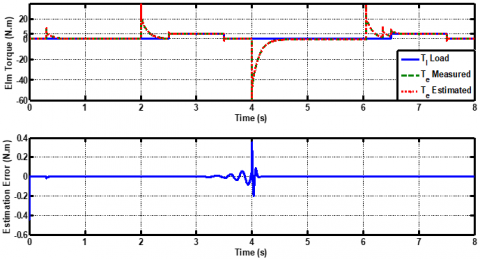
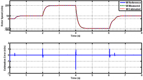
Figures 2 and 3 show the electromechanical torque and the rotor angular speed variations respectively, with respect to the simulation tests.
The variation profile is:
The load torque Tl = 5 Nm introduced at time t = 2.5 Sec and 6.5 Sec. In parallel, the machine undergoes a variation of the angular speed w_ref =50 rd/s (low speed), w_ref =220 rd/s (high speed), w_ref =-157 rd/s (speed inversion) and w_ref =50 rd/sfrom t = 0.5 Sec, 2 sec, 4 Sec and 6 Sec respectively. From Figures 2 and 3, it is clear that the estimated state variables thoroughly follow the desired trajectories of the induction motor.
The rotor flux modulus is given by Figure 4. We can notice that the flux reaches its reference value without any overshoot or oscillations.
The results of the simulation obtained from the Figures 3 and 4 illustrate that all the parameters of the (IM) are changed following the variations imposed by the load torque Figure 2.
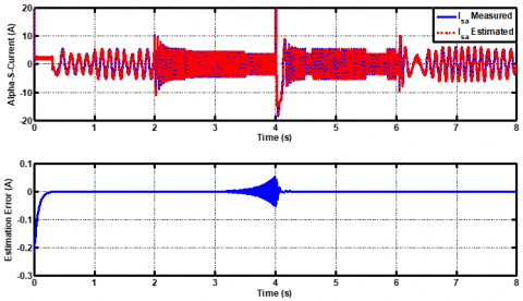
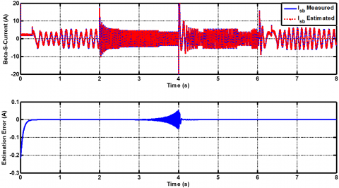
The measured and estimated components (alpha, beta) of stator currents are given by Figures 5 and 6 respectively. It is clear that these estimated parameters of the induction motor perfectly follow the desired trajectories.
From the results obtained, it is noted that the system-based nonlinear observer efficiently estimates the unmeasured state variables of (IM). Moreover, these estimated parameters follow the imposed variations of the load torque while respecting the proposed control law.
Figure 2. Load, Measured and estimated Electromechanical Torque
Figure 3. Rotor speed (Reference measured and estimated) evolution according to load variations
Figure 4. Rotor flux norm modulus (reference measured and estimated) and estimation error
Figure 5. Alpha-stator current components and its estimation error
Figure 6. Beta-stator current components and its estimation error
In this article, we have studied a sensorless control strategy for the induction motor (IM) using a Backstepping control and a nonlinear observer based on the circle-criterion method.
The proposed scheme has been introduced to solve the problem of non-linearities of the system, ensure good performance for the trajectory tracking, improve reliability in case of uncertainties of the system and load disturbance rejection.
Obtained simulation results illustrate that this suggested scheme ensures a perfect control regardless of the profile trajectories physically imposed on the induction motor. It has been proven that the suggested backstepping control offers satisfactory results in terms of velocity and flux reference tracking and load disturbance rejection. The implementation of a nonlinear observer has participated effectively to estimate the non-measurable parameters that are necessary for the nonlinear control. However, it introduces linear matrix inequality (LMI) conditions.
This work is supported by the Directorate General of Scientific Research and Technological Development (DGRSDT) of Algeria.
[1] Bensaker, B., Kherfane, H., Metatla, A., Wamkeue, R. (2003). State space modelling of induction motor for sensorless control and monitoring purposes. International-Journal Electromotion, 10(4): 483-488.
[2] Abdelati, R., Mimouni, M.F. (2019). Optimal control strategy of an induction motor for loss minimization using Pontryaguin principle. European Journal of Control, 49: 94-106. https://doi.org/10.1016/j.ejcon.2019.02.004
[3] Utkin, V.I. (1993). Sliding mode control design principles and applications to electric drives. IEEE Transactions on Industrial Electronics, 40(1): 23-36. https://doi.org/10.1109/41.184818
[4] Yousef, H.A., Wahba, M.A. (2009). Adaptive fuzzy mimo control of induction motors. Expert Systems with Applications, 36(3): 4171-4175. https://doi.org/10.1016/j.eswa.2008.04.004
[5] Berrezzek, F., Bourbia, W., Bensaker, B. (2016). Flatness based nonlinear sensorless control of induction motor systems. International Journal of Power Electronics and Drive Systems, 7(1): 265-278. https://doi.org/10.11591/ijpeds.v7.i1.pp265-278
[6] Fattahl H.A.A., Loparo K.A. (2000). Passivity-based torque and flux tracking for induction motors with magnetic saturation. Proceedings of the American Control Conference, Chicago, Illinois, pp. 0-4.
[7] Ferrara, A. (2007). Discussion on: “An adaptive variable structure control law for sensorless induction motors”. European Journal of Control, 13(4): 393-397. https://doi.org/10.3166/ejc.13.393-397
[8] Bouhoune, K., Yazid, K., Boucherit, M.S., Chériti, A. (2017). Hybrid control of the three phase induction machine using artificial neural networks and fuzzy logic. Applied Soft Computing, 55: 289-301. https://doi.org/10.1016/j.asoc.2017.01.048
[9] Fateh, M., Abdellatif, R. (2017). Comparative study of integral and classical backstepping controllers in IFOC of induction motor fed by voltage source inverter. International Journal of Hydrogen Energy, 42(28): 17953-17964. https://doi.org/10.1016/j.ijhydene.2017.04.292
[10] Trabelsi, R., Khedher, A., Mimouni, M.F., M'sahli, F. (2012). Backstepping control for an induction motor using an adaptive sliding rotor-flux observer. Electric Power Systems Research, 93: 1-15. https://doi.org/10.1016/j.epsr.2012.06.004
[11] Mehazzem, F., Nemmour, A.L., Reama, A. (2017). Real time implementation of backstepping-multiscalar control to induction motor fed by voltage source inverter. International Journal of Hydrogen Energy, 42(28): 17965-17975. https://doi.org/10.1016/j.ijhydene.2017.05.035
[12] Bourbia, W., Berrezzek, F., Bensaker, B. (2014). Circle-criterion based nonlinear observer design for sensorless induction motor control. International Journal of Automation and Computing, 11(6): 598-604. https://doi.org/10.1007/s11633-014-0842-1
[13] Ţiclea, A., Besançon, G. (2006). Observer scheme for state and parameter estimation in asynchronous motors with application to speed control. European Journal of Control, 12(4): 400-412. https://doi.org/10.3166/ejc.12.400-412
[14] Atassi, A.N., Khalil, H.K. (2000). Separation results for the stabilization of nonlinear systems using different high-gain observer designs. Systems & Control Letters, 39(3): 183-191. https://doi.org/10.1016/S0167-6911(99)00085-7
[15] Zemouche, A., Boutayeb, M. (2013). On LMI conditions to design observers for Lipschitz nonlinear systems. Automatica, 49(2): 585-591. https://doi.org/10.1016/j.automatica.2012.11.029
[16] Beikzadeh, H., Taghirad, H.D. (2012). Exponential nonlinear observer based on the differential state-dependent Riccati equation. International Journal of Automation and Computing, 9(4): 358-368. https://doi.org/10.1007/s11633-012-0656-y
[17] Liu, L.P., Fu, Z.M., Song, X.N. (2012). Sliding mode control with disturbance observer for a class of nonlinear systems. International Journal of Automation and Computing, 9(5): 487-491. https://doi.org/10.1007/s11633-012-0671-z
[18] Moutchou, M., Abbou, A., Mahmoudi, H. (2012). Sensorless speed backstepping control of induction machine, based on speed MRAS observer. 2012 International Conference on Multimedia Computing and Systems, Tangiers, Morocco, pp. 1019-1024. https://doi.org/10.1109/ICMCS.2012.6320166
[19] Djeghali, N., Ghanes, M., Barbot, J.P., Djennoune, S. (2011). Sensorless fault tolerant control based on backstepping strategy for induction motors. IFAC Proceedings Volumes, 44(1): 6154-6159. https://doi.org/10.3182/20110828-6-IT-1002.01943
[20] Ting, C.S., Chang, Y.N. (2013). Observer-based backstepping control of linear stepping motor. Control Engineering Practice, 21(7): 930-939. https://doi.org/10.1016/j.conengprac.2013.02.018
[21] Abdelhak, B., Bachir, B. (2015). A high gain observer based sensorless nonlinear control of induction machine. International Journal of Power Electronics and Drive Systems, 5(3): 305-314. https://doi.org/10.11591/ijpeds.v5.i3.pp305-314
[22] Arcak, M., Kokotović, P. (2001). Nonlinear observers: a circle criterion design and robustness analysis. Automatica, 37(12): 1923-1930. https://doi.org/10.1016/S0005-1098(01)00160-1
[23] Arcak, M. (2005). Certainty-equivalence output-feedback design with circle-criterion observers. IEEE Transactions on Automatic Control, 50(6): 905-909. https://doi.org/10.1109/TAC.2005.849257
[24] Ibrir, S. (2007). Circle-criterion approach to discrete-time nonlinear observer design. Automatica, 43(8): 1432-1441. https://doi.org/10.1016/j.automatica.2007.01.012
[25] Berrezzek, F., Bensaker, B. (2019). A comparative study of nonlinear circle criterion based observer and H∞ observer for induction motor drive. International Journal of Power Electronics and Drive System, 10(3): 1229-1243. https://doi.org/10.11591/ijpeds.v10.i3.1229-1243