Mouna Tali* | Ahmed Essadki | Tamou Nasser
© 2021 IIETA. This article is published by IIETA and is licensed under the CC BY 4.0 license (http://creativecommons.org/licenses/by/4.0/).
OPEN ACCESS
To enhance the power quality in electric power systems, active power filter can be successfully used for harmonics mitigation and reactive power compensation. In this paper, a new approach using novel direct power control PDPC based on grid voltages estimation is proposed to improve the dynamic performance of shunt active power filter and reduce the system cost and robustness by minimizing the number of sensors in grid connected PV system. The grid voltages are estimated online by using an adaptive linear neural network (ADALINE) and the proposed PDPC is based on the extended pq theory. According to the simulation results, the proposed control strategy using a voltage estimator instead of voltage sensors not only reduce the size and cost but the reliability of the active power filter PV-APF is improved under normal and severe grid voltage conditions.
APF, PV system, nonlinear load, neural adaptive filter, Adaline, direct power control, THD
Harmonic pollution in electrical power systems caused by extensive use of nonlinear loads is one of the most serious power quality problems that have great concern and attract researchers interests. The presence of harmonics and reactive power cause several harmful effects such as power losses, malfunction of the grid equipments. These problems can lead to degradation of the system efficiency (indicated by low power factor). As a result, it is prerequisite to compensate harmonics and reactive powers to develop unity power factor and avoid unwanted losses [1]. Basically, there are two kinds of compensators: passive power filters (PPFs) and active power filters (APFs), the first PPFs have been considered as a good alternative for harmonics compensation due to its low cost, simplicity and high efficiency [2], however, PPFs have many disadvantages such as large size, instability and resonance with loads and/or source impedance, in addition, the PPF cannot to be adapted to the dynamic changes of the nonlinear loads. That is why PPFs are gradually replaced by active power filters APFs. APFs have the capability to overcome the above-mentioned disadvantages inherent in PPFs and have become an alternative solution to improve power quality. Among various APF configurations [3], the shunt APF is the most popular active filter and widely used in electric power systems. Recently, in the grid-connected photovoltaic PV system, power quality issues have been resolved by the use of the multifunctional PV inverter acting as active power filter APF which can inject active power and mitigate the harmonics [4]. Several control strategies have been proposed to extract and estimate the harmonic currents like FFT technique, p-q theory, Synchronous d-q reference frame theory [5]. Many works, on harmonics elimination in SAPF such as sliding mode control, neural network control, and fuzzy control are discussed in refs. [6-8]. A model based on Direct Power Control DPC for three-phase shunt active power filtering in grid connected PV system, is proposed to eliminate line current harmonics and compensate reactive power [9]. Neural network-based intelligent control strategies have been developed to alleviate quality problems [10]. Generally, in the conventional APF controllers three types of sensors are required; current sensors; source voltage sensors and dc-bus voltage sensor. Hence, to reduce the cost, system complexity and sensor noise while retaining the system performance and reliability, some sensors can be emulated. The first and the third sensors are indispensables regarding system control, and system protection against overcurrent and dc-side overvoltage. However, the ac-voltage sensors can be eliminated and estimated from other measured quantities such as the currents and the DC-link voltage [11].
Several control strategies based on voltage estimation have been proposed in the literature. The grid voltages are estimated using disturbance observer (DOB) in the stationary reference frame [12]. The voltages are calculated from the estimated instantaneous active and reactive powers for PWM converters [13], other techniques utilized the measured currents and converter parameters in order to estimate grid voltages are discussed in ref. [14]. A nonlinear Luenberger type observer has been presented to eliminate the line voltage sensors [15]. Abouelmahjoub et al. [16] proposes an adaptive observer estimating the grid voltages and impedances parameters in three phase shunt active power filter SAPF. In others works, fuzzy logic and neural network are utilized to estimate unknown parameters without detail information [17-20].
The goal is to ensure satisfactory compensation performance at difficult situations. However, the majority of the previous controllers present instability under unbalanced grid voltages, which decrease their efficiency and reliability.
This paper addresses this problem by proposing an adaptive neural-network voltage estimator for a SAPF control operating in an unbalanced system, the control strategy utilize a novel DPC method based on extended pq theory. The proposed algorithm provides low complexity design structure and ensure a satisfactory compensation.
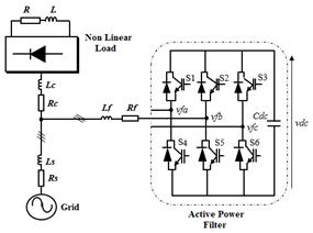
The SAPF structure is based on voltage-source inverter with only a single capacitor in the DC side as shown in Figure 1; it is connected in parallel with the nonlinear load. SAPF injects compensating currents at the PCC which have the same magnitude but opposite in phase of the harmonic currents drawn by the nonlinear loads, as a result, the source currents can be balanced, sinusoidal and in phase with the source voltages.
Figure 1. Topology of active power filter
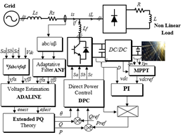
The proposed SAPF configuration based on the new DPC control and neural network voltage estimator in this work is shown in Figure 2. The considered load to evaluate the effectiveness of the SAPF is three-phase rectifier with R-L load.
Figure 2. Structure of PV-SAPF integrated based on voltage estimator with DPC Control strategy
Direct power control DPC proposed by Nogushi has become an interesting control strategy of Active power filter. The converter switching states are selected from a switching table based on errors of active and reactive powers and the vector voltage position without any inner current control and PWM modulator. The active power reference is obtained from an outside DC voltage PI controller, the reactive power must be kept to zero value to achieve unity power factor. These references are compared with the calculated P and Qnov values given by Eq. (4), in reactive and active power hysteresis controllers, respectively.
Figure 3. Equivalent circuit topology
Figure 3 shows the equivalent circuit of the SAPF connected to the grid and the nonlinear load per phase, the expression of grid voltage eαβ with respect to grid current is αβ and converter voltage vfαβ is given by:
$e_{\alpha \beta}=L_{s} \frac{d i_{s \alpha \beta}}{d t}+v_{f \alpha \beta}+L_{f} \frac{d i_{s \alpha \beta}}{d t}$ (1)
Voltage vectors generated by the inverter, when expressed in terms of the switching states and the dc link voltage is:
$v_{f \alpha \beta}=\sqrt{\frac{2}{3} V_{d c}\left(S_{a}+S_{b} e^{j\left(\frac{2 \pi}{3}\right)}+S_{c} e^{j\left(\frac{4 \pi}{3}\right)}\right)}$ (2)
where, Sa, Sb and Sc are the switching states at each leg of the inverter:
$S_{a}=\left\{\begin{array}{ll}1, & \text { if } S_{1} O N \text { and } S_{4} O F F \\ 0, & \text { if } S_{1} O F F \text { and } S_{4} O N\end{array}\right.$
$S_{b}=\left\{\begin{array}{ll}1, & \text { if } S_{2} O N \text { and } S_{5} O F F \\ 0, & \text { if } S_{2} O F F \text { and } S_{5} O N\end{array}\right.$
$S_{c}=\left\{\begin{array}{ll}1, & \text { if } S_{3} O N \text { and } S_{6} O F F \\ 0, & \text { if } S_{3} O F F \text { and } S_{6} O N\end{array}\right.$
It is worth noting that both the grid voltages and grid currents are expressed in stationary reference frame is given by:
$\left[\begin{array}{l}e_{\alpha} \\ e_{\beta}\end{array}\right]=\sqrt{\frac{2}{3}}\left[\begin{array}{ccc}1 & -\frac{1}{2} & -\frac{1}{2} \\ 0 & \frac{\sqrt{3}}{2} & -\frac{\sqrt{3}}{2}\end{array}\right]\left[\begin{array}{l}e_{s a} \\ e_{s b} \\ e_{s c}\end{array}\right]$ (3)
The conventional DPC strategy based on original pq theory gives satisfactory performances as long as the supply voltage is ideal, but when this condition is not verified and distortion or unbalance affect the grid voltages, the performance will degrade severely, for this reason, the motivation in this paper is to extended the performance of DPC to be operate under unbalanced grid voltages. So, the incompetency of the conventional DPC under unbalanced grid voltages has prompted an initial employment of the extension pq theory by Komatsu et al.
In the extended power theory, the instantaneous active and the novel reactive power Qnov can be expressed as [13]:
$\left(\begin{array}{c}P \\ Q^{n o v}\end{array}\right)=\left(\begin{array}{c}e_{\alpha} i_{s \alpha}+e_{\beta} i_{s \beta} \\ e_{\alpha}^{\prime} i_{s \alpha}+e_{\beta}^{\prime} i_{s \beta}\end{array}\right)$ (4)
where, the grid voltage e'αβ denote the quadrature voltage e lagging eα and eβ by 90 degrees respectively. It is important to mention that with this novel reactive power, the performance under both sinusoidal, unbalanced grid voltages are not affected, and sinusoidal currents are obtained.
Reconsidering equation 4 the active power derivative and novel reactive power derivative are given by:
$\frac{d p}{d t}=e_{\alpha} \frac{d i_{s \alpha}}{d t}+i_{s \alpha} \frac{d e_{\alpha}}{d t}+e_{\beta} \frac{d i_{s \beta}}{d t}+i_{s \beta} \frac{d e_{\beta}}{d t}$ (5)
$\frac{d q^{\text {nov }}}{d t}=e_{\alpha}^{\prime} \frac{d i_{s \alpha}}{d t}+i_{s \alpha} \frac{d e_{\alpha}^{\prime}}{d t}+e_{\beta}^{\prime} \frac{d i_{s \beta}}{d t}+i_{s \beta} \frac{d e_{\beta}^{\prime}}{d t}$ (6)
The derivate of voltages and currents can be expressed as:
$\frac{d e_{\alpha}}{d t}=-\omega e_{\beta} ; \frac{d e_{\beta}}{d t}=+\omega e_{\alpha} ; \frac{d e^{\prime}}{d t}=\omega$ (7)
$\frac{d i_{s}^{\alpha \beta}}{d t}=\frac{1}{L_{s}+L_{f}}\left(e^{\alpha \beta}-v_{f}^{\alpha \beta}\right)$ (8)
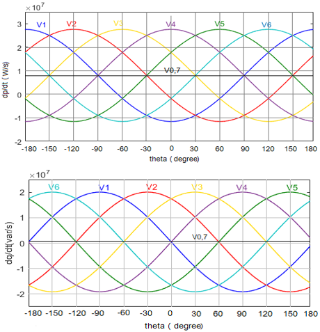
According to Eqns. (5) to (12), the variation of active and the novel reactive power for different converter voltage vectors can be calculated and illustrated in Figure 4. Only one optimal inverter voltage vector which leads to the minimum powers variation, will be selected.
The VDC is the dc link voltage and Vf is the converter voltage vector Vf=2/3Vdc e(j π/3(n-1)) (n=1, 2, …, 6), e=‖eαβ‖ and θ is the angular position of the grid voltage vector in αβ coordinates defined as:
$\theta=\operatorname{artan}^{-1}\left(\frac{e_{\beta}}{e_{\alpha}}\right)$ (9)
$\frac{d p}{d t}=K\left(K^{\prime}-\cos \left(\theta-(n-1) \frac{\pi}{3}\right)\right)-\omega q$ (10)
$\frac{d q^{n o v}}{d t}=-K\left(\sin \left(\theta-(n-1) \frac{\pi}{3}\right)\right)+\omega p$ (11)
where, $K=\frac{\|e\|}{L_{s}+L_{f}} \sqrt{\frac{2}{3}} V_{d c}, K^{\prime}=\frac{\|e\|^{2}}{L_{s}+L_{f}}$.
Figure 4. Instantaneous power variations for different voltage vectors
The optimal inverter voltage vector can be selected to adjust the active power and the reactive power from the new switching table which elaborated depending the output of the hysteresis comparators dp, dq and the voltage vector position as defined as:
$(n-1) \frac{\pi}{6} \leq \theta_{n} \leq n \frac{\pi}{6}$ (12)
$d p=\left\{\begin{array}{l}1 \text { if Pref }-P \geq h p \\ 0 \text { if Pref }-P \leq h p\end{array}\right.$
$d q=\left\{\begin{array}{l}1 \text { if Qref }-Q \geq h p \\ 0 \text { if Qref }-Q \leq h p\end{array}\right.$
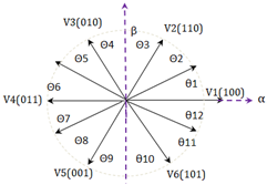
For this purpose, the working plane (α, β) is divided in 12 sectors (see Figure 5):
Figure 5. Sectors classification for DPC in stationary αβ frame
Pref is controlled from an outer loop, so the dc link voltage of VSI is measured and compared with the reference dc link voltage which output from the MPPT algorithm, a traditional PI algorithm is used for better regulation and the pref represents the output of the pi controller, and the reactive power is controlling to be zero to achieve unity power factor.
To obtain the switching table for the DPC control, four combinations of active and reactive power variation are available and by examining Figure 4, we can see that are several voltage vector possibilities for a particular combination of power variation for each angular position. However, only one suitable voltage vector should be chosen for a particular combination of power variation which produce much lower active power and reactive power variation (dp/dtmin) and (dq/dtmin) to minimize the errors between reference and the measured active power and reactive power.
Table 1. Proposed DPC
|
dp |
dq |
θ1 θ2 θ3 θ4 θ5 θ6 θ7 θ8 θ9 θ10 θ11 θ12 |
|
0 0 1 1 |
0 1 0 1 |
v1 v1 v2 v2 v3 v3 v4 v4 v5 v5 v6 v6 v2 v2 v3 v3 v4 v4 v5 v5 v6 v6 v1 v1 v5 v6 v6 v1 v1 v2 v2 v3 v3 v4 v4 v5 v3 v4 v4 v5 v5 v6 v6 v1 v1 v2 v2 v3 |
In this paper, active and reactive power based DPC controller are calculated by using the estimated grid voltages in the αβ frame. For removing the ac voltage sensors, the grid voltage is obtained in terms of the inverter voltage and the source current as shown below:
$e_{\alpha \beta}=L \frac{d i_{s \alpha \beta}}{d t}+v_{f \alpha \beta}$
where, L=Ls+Lf.
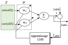
The developed grid voltages estimator is depicted in Figure 6, the Adaline algorithm is used to extract the fundamental component using least-mean-square (LMS) algorithm as its learning rule to update the weight W. To help to give a good estimation, the source currents which can be affected by noises and harmonics will be filtered by an adaptive neural filter ANF (bloc diagram of the adaptive neural network). The adaptive linear algorithm ADALINE introduced by Widrow Hoff based on LMS learning rule represents now an efficient approach for fast prediction and estimation of signal parameters. Due to its simple structure and the capability, self-adapt on line.
Figure 6. Proposed grid voltage estimator
The designing methodology supposes that the voltage/current can be represented by the sum of a fundamental frequency and multiple of fundamental frequency components which can be written as:
$y_{\alpha}(k)=\sum_{n=1}^{N} Y_{n} \cos \left(\omega_{n} k T_{S}+\varphi_{n}\right)=$$Y_{1} \cos \left(\omega_{1} k T_{s}+\varphi_{1}\right)+\sum_{n=2}^{\infty} Y_{n} \cos \left(Y_{n} k T_{s}+\varphi_{n}\right)$
$y_{\beta}(k)=\sum_{n=1}^{N} Y_{n} \sin \left(\omega_{n} k T_{S}+\varphi_{n}\right)=$$Y_{1} \sin \left(\omega_{1} k T_{s}+\varphi_{1}\right)+\sum_{n=2}^{\infty} Y_{n} \sin \left(Y_{n} k T_{s}+\varphi_{n}\right)$ (13)
where, eαβ=yαβ, ωn, An and φn are pulsation, amplitude and phase angle.
The process of the line voltage estimator is similar to that of the adaptive filter, which extracts fundamental components and neglects all harmonic components greater than 1.
The estimated grid voltage using ADALINE process can be expressed as:
$y_{\alpha}(k)=Y_{1} \cos \left(\omega_{1} k T_{s}+\varphi_{1}\right)$
$y_{\beta}(k)=Y_{1} \sin \left(\omega_{1} k T_{s}+\varphi_{1}\right)$ (14)
$y_{\alpha}(k)=Y_{1} \cos \varphi_{1} \cos \left(\omega_{1} k T_{s}\right)$$-Y_{1} \sin \varphi_{1} \sin \left(\omega_{1} k T_{s}\right)$
$y_{\beta}(k)=Y_{1} \cos \varphi_{1} \sin \left(\omega_{1} k T_{s}\right)$$+Y_{1} \sin \varphi_{1} \cos \left(\omega_{1} k T_{s}\right)$ (15)
So, in vectorial notation the estimated grid voltage using ADALINE process can be written as:
$e_{\alpha \beta}=y_{\alpha \beta e s t}(k)=W^{T} X(k)$ (16)
where, X(k)=[cos(ω1kTs)sin(ω1kTs)]T.
$W_{\alpha}=\left[\begin{array}{ll}w_{1 \alpha} & w_{2 \alpha}\end{array}\right]=\left[Y_{1} \cos \varphi_{1}-Y_{1} \sin \varphi_{1}\right]$
$W_{\beta}=\left[\begin{array}{ll}w_{1 \beta} & w_{2 \beta}\end{array}\right]=\left[\begin{array}{ll}Y_{1} \sin \varphi_{1} & Y_{1} \cos \varphi_{1}\end{array}\right]$ (17)
where, X(k) is the reference input vector of the ADALINE and the W represents the weight vector whose are updated by using the adaptive learning process.
The LMS algorithm is used as learning rule in order to minimize the error ξ(k), the learning rule can be expressed as:
$W(k+1)=W(k)+\mu \xi(k) X(k)$ (18)
where, μ is the learning factor, ξ(k) is the estimation error.
$\xi(k)=y(k)-y_{e s t}(k)$ (19)
Thus, at each iteration, with the supervised learning process of ADALINE LMS, neural filter parameters (adaptive neural network diagram) are updated to make the above error can asymptotically converge to zero. And the estimated output yest(k) behavior becomes close to set of desired output y(k).
An algorithm with a high rate of convergence, stability and good tracking ability is required. The optimization method widely used for many identification applications is the gradient descent technique but it has the drawback of having a very slow convergence rate, however, the Least Mean Square (LMS) algorithm developed by Widrow-Hoff became the most used adaptive algorithm due to its simplicity of calculation and its proven robustness.
In order to enhance the precision of the proposed ADALINE voltage estimator, the weights updating are adjusted using the learning rate μ (0<μ<2 [20]) (μ=0, 2 is chosen in order to have a faster algorithm and ensure good convergence).
The stability of the proposed algorithm is proved using Lyapunov's theory [20].
A candidate Lyapunov function satisfying the learning rule (13) above, is proposed as:
$V(k)=\xi^{2}(k)+\xi^{2}(k-1)$ (20)
$V(k)=\beta^{k} \xi^{2}(k)$ (21)
where,
$\beta^{k}=\left(1+\frac{\xi^{2}(k-1)}{\xi^{2}(k)}\right)$ (22)
The Lyapunov stability conditions are:
$\left\{\begin{array}{c}V(k)>0 \\ V(k)-V(k-1)=\Delta V(k)<0\end{array}\right.$ (23)
ΔV(k) can be evaluated as:
$\Delta V(k)=\beta_{k}\left[d(k)-W^{T}(k) x(k)\right]^{2}-\beta_{k} \xi^{2}(k-1)$ (24)
$\Delta V(k)=-\beta_{k} \xi^{2}(k-1)<0$ (25)
According to (20) the tracking error can converge to zero, hence the stability condition is satisfied (see Appendix A).
The PV generator behaving as a power source for the SAPF, is drained by the boost converter of the photovoltaic panel with a maximum power point tracking control (MPPT) using the Perturb and Observe (P&O) algorithm. Therefore, in order to regulate the voltage of the DC link and compensate for the losses of the system under all conditions, a simple PI controller is proposed, the gains Kp and Ki are calculated and adjusted according to the dynamic response.
The performance of the proposed neural network voltage estimator with PV-SAPF controller employing a novel DPC method has been evaluated through simulation using MATLAB/SIMULINK. The challenge of the whole system is to achieve sinusoidal and balanced grid current under balanced and unbalanced supply condition and varying irradiance. To verify the behavior of SAPF in grid connected PV-system, an irradiation profile showed in Figure 10(a) is proposed. For modeling the PV system, the ESPMC270 panel is utilized, the key specification are shown in Table 2. And Table 3 illustrates simulation parameters.
Table 2. ESPMC270 PV panel parameters
|
Description |
Value |
|
Ideality factor Maximum Power Short-circuit current Open circuit voltage Parallel connected modules Serie connected cells |
a=1.3 Pmax=270W Isc=8.2A Voc=21.06V Np=2 Ns=15 |
Table 3. List of each component used for the proposed SAPF
|
Parameters |
Values |
|
es, fs, |
100 v,50 Hz |
|
Ls, Rs |
10 µH, 0.1 Ω |
|
LL, RL |
10 mH, 30 Ω |
|
Lf, Rf, |
8 mH, 0.01 Ω |
|
Cdc Vdc |
2200 µF, 300 v |
|
Kp, Ki |
2, 0.008 |
6.1 Case 1 balanced grid voltages
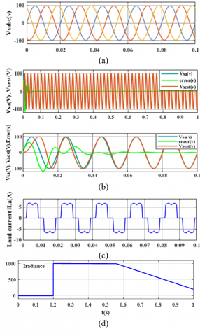
The actual and estimated grid voltages are given in Figures 7(a) and (b), it can be observed that at the steady state the waveforms of the estimated grid voltage and actual one are very close with minimum estimation errors.
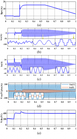
Figure 8 shows the simulation results under balanced and sinusoidal grid voltages for the proposed DPC using the extended pq theory, in this case, without SAPF compensation, the source currents are distorted severely with the THD around to 27.28%. At t=0.1 s, SAPF starts to compensate harmonics, and the source current becomes sinusoidal and in phase with the grid voltage and the THD current reduces to 1.01% at 0 W/m², (1.57% at 200 W/m² and 2.47% at 1000 W/m²), the compensating current injected by the SAPF at the PCC is depicted in Figure 8(b). Reduction in the THD means that the proposed controller has better steady-state response, which confirms the effectiveness of the control method in varying solar irradiation.
Figure 7. (a) Grid voltages, (b) Estimated grid Voltage and actual grid voltage and estimation error in steady state and in transitional state, (c) Load current, (d) Irradiance profile
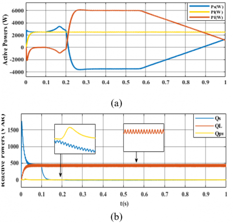
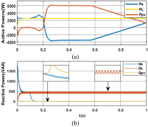
The active and reactive powers of the whole system are depicted in Figure 9 showing successful transfer of power from the PV-SAPF to the grid and to the load under steady-state condition. When active power is injected from the PV system (1000 W/m²), the source current is decreased and will be in opposite in phase with the grid voltage, this means that the PV power is higher than the power demanded by the load.
Figure 8(e) illustrates the dc link voltage Vdc, it maintains its reference perfectly at different irradiations, at t=0.2 s, oscillation can be observed due to exchange of powers between the grid and PV system under rapidly change of irradiation, in the same time p and q are well controlled to their references. Figure 9 (a) shows the successful transfer of power from the PV-SAPF to the grid and PV-SAPF power is exactly equal to the sum of the source power and load power under steady-state and in Figure 9(b), negligible reactive power Qs (extended pq theory)with a few oscillations in the steady state, confirms the operation at unity PF. Consequently, the proposed control strategy based on the neural network voltage estimator presents a good stability and best performance
Figure 8. (a) PV current, (b) compensating current, (c) source current, (d) source voltage and source current, (e) DC link voltage
Figure 9. (a) Active powers, (b) Reactive powers
6.2 Case 2 unbalanced grid voltages
To verify the performance of the developed neural network voltage estimator, an unbalanced system is applied, the magnitudes of phases B and C are 80% of the magnitude of phase A, as depicted in Figure 10(a). In Figure 10(b), the actual and estimated grid voltage are presented under unbalanced grid voltages sag, according the obtained results, the neural network estimator is not affected and is stable, the actual and estimated grid voltages stay close with an acceptable error in steady state as shown in Figure 10(c).
Figure 10. (a) Unbalanced grid voltages, (b) Estimation grid voltage, (c) actual voltage and estimation error
Figure 11. (a) source currents, (b) source current with grid voltage in phase a
The proposed PDPC algorithm behavior in this case is shown in Figures 11. Thanks to the extended pq theory good results are obtained under unbalanced grid voltage, it is observed in Figure 11(a) that the source currents are balanced and have the same magnitude during a solar irradiation changing, The THD is improved to a lower values (2.44% at 0 W/m², 2.55% at 200 W/m² and 5.66% at 1000 W/m²). In Figure 12(a), it can be not supply local loads but also it can inject the surplus of the power to the grid at the fort irradiation (G=1000 w/m²) and in Figure 12(b), it is observed that the new reactive power stills constant and tracks its reference (0 VAR) to achieve unity power factor under unbalanced voltage conditions.
Figure 12. (a) Active Powers, (b) Reactive Powers
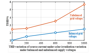
Figure 13 illustrates the current THD of the PDPC based on the extended theory under the balance and unbalance grid voltage. The performance of the proposed and developed control method is determined by significant reduction in the THD, meanwhile, under unbalanced voltages the THD of current increased slightly, but it still remained within the limits of the IEEE-519 standard as seen in Table 4.
Figure 13. THD variation under solar irradiation variation
Table 4. Current THD under balanced and unbalanced grid voltages
|
THD |
APF off |
APF on |
||
|
Solar Irradiation |
|
0W/m² |
200W/m² |
1000W/m² |
|
Balanced grid |
27.28% |
1.01% |
1.57% |
2.47% |
|
Unbalanced grid |
27.52% |
2.44% |
2.55% |
5.66% |
In this paper, a new voltage sensorless control strategy is developed for shunt active power filter in grid connected PV system, this control method is based on a neural voltage estimator using ADALINE network. Good dynamic performance, stability and strong robustness under different aspects are proven in dynamic operation and during steady state. The Lyapunov stability theorem has been exploited to ensure the convergence and stability of the proposed control performance.
The simulation results confirm that the proposed Adaline estimator algorithm, using the proposed DPC based on extended PQ theory represents high accuracy of harmonics mitigation with significant reduction of THD. In addition, it has also able to maintain the balanced grid current under unbalanced grid voltage as well as in changed solar irradiation.
$\Delta V(k)=\beta_{k}\left[d(k)-W^{T}(k-1) x(k)-\mu \xi^{T}(k) x^{T}(k) x(k)\right]^{2}$$\quad-\beta_{k} \xi^{2}(k-1)$
$\Delta V(k)=\beta_{k}\left[d(k)-W^{T}(k-1) x(k)-\Delta W^{T}(k) x(k)\right]^{2}$$\quad-\beta_{k} \xi^{2}(k-1)$
where,
$y(k)=W_{o p}^{T}(k) x(k)$
$\Delta V(k)=\beta_{k}\left[W_{o p}^{T}(k) x(k)-W^{T}(k-1) x(k)\right.$$\left.-\Delta W^{T}(k) x(k)\right]^{2}-\beta_{k} \xi^{2}(k-1)$
$\Delta V(k)=\beta_{k}\left[\Delta W_{o p}^{T}(k) x(k)-\Delta W^{T}(k) x(k)\right]^{2}$$-\beta_{k} \xi^{2}(k-1)$
When $k \rightarrow \infty W^{T}(k)=W_{o p}^{T}(k)$, then
$W_{o p}^{T}(k)-W^{T}(k-1)=W^{T}(k)-W^{T}(k-1)$
$\lim _{k \rightarrow \infty}\left[\Delta W_{o p}^{T}(k) x(k)-\Delta W^{T}(k) x(k)\right]^{2}=0$, and
$\lim _{k \rightarrow \infty} \beta^{k}=2>0, \lim _{k \rightarrow \infty} \beta^{k}\left(1+\frac{\xi^{2}(k-1)}{\xi^{2}(k)}\right)=2$
|
e |
Source Voltage |
|
is |
Source Current |
|
iL iF |
Load Current Filter compensator Current |
|
Ls Lf LL Vdc Cdc PV SAPF THD P/Q |
Source-side inductor Inductor filter Load side inductor Dc-link Voltage Dc-link capacitor Photovoltaic Shunt Active Power Filter Total Harmonic Filter Active and Reactive Power |
|
Greek symbols |
|
|
ξ |
Estimator Error |
|
µ |
Learning Factor |
[1] Saribulut, L., Teke, A., Meral, M., Tumay, M. (2011). Active power filter: Review of converter topologies and control strategies. Gazi University Journal of Science, 24(2): 283-289.
[2] Tali, M., Obbadi, A., Elfajri, A., Errami, Y. (2014). Passive filter for harmonics mitigation in standalone PV system for non linear load. In 2014 International Renewable and Sustainable Energy Conference (IRSEC), Ouarzazate, Morocco, pp. 499-504. https://doi.org/10.1109/IRSEC.2014.7059834
[3] Nie, X., Liu, J. (2019). Current reference control for shunt active power filters under unbalanced and distorted supply voltage conditions. IEEE Access, 7: 177048-177055. https://doi.org/10.1109/ACCESS.2019.2957946
[4] Aredes, M., Akagi, H., Watanabe, E.H., Salgado, E.V., EncarnaÇÃo, L.F. (2009). Comparisons between the p--q and p--q--r theories in three-phase four-wire systems. IEEE Transactions on Power Electronics, 24(4): 924-933. https://doi.org/10.1109/TPEL.2008.2008187
[5] Zeng, Z., Yang, H., Guerrero, J.M., Zhao, R. (2015). Multi-functional distributed generation unit for power quality enhancement. IET Power Electronics, 8(3): 467-476. https://doi.org/10.1049/iet-pel.2013.0954
[6] Sahara, A., Kessal, A., Rahmani, L., Gaubert, J.P. (2016). Improved sliding mode controller for shunt active power filter. Journal of Electrical Engineering and Technology, 11(3): 662-669. https://doi.org/10.5370/JEET.2016.11.3.662
[7] Fogli, G.A., de Almeida, P.M., Rodrigues, V.M., Barbosa, P.G. (2015). Sliding mode control of a shunt active power filter with indirect current measurement. In 2015 IEEE 13th Brazilian Power Electronics Conference and 1st Southern Power Electronics Conference (COBEP/SPEC), Fortaleza, Brazil, pp. 1-5. https://doi.org/10.1109/COBEP.2015.7420051
[8] Salam, A.A., Ab Hadi, N.A. (2014). Fuzzy logic controller for shunt active power filter. In 2014 4th International Conference on Engineering Technology and Technopreneuship (ICE2T), Kuala Lumpur, Malaysia, pp. 256-259. https://doi.org/10.1109/ICE2T.2014.7006258
[9] Boukezata, B., Chaoui, A., Gaubert, J.P., Hachemi, M. (2016). Power quality improvement by an active power filter in grid-connected photovoltaic systems with optimized direct power control strategy. Electric Power Components and Systems, 44(18): 2036-2047. https://doi.org/10.1080/15325008.2016.1210698
[10] Abdeslam, D.O., Wira, P., Mercklé, J., Flieller, D., Chapuis, Y.A. (2007). A unified artificial neural network architecture for active power filters. IEEE Transactions on Industrial Electronics, 54(1): 61-76. https://doi.org/10.1109/TIE.2006.888758
[11] Bai, H., Wang, X., Blaabjerg, F. (2017). A grid-voltage-sensorless resistive-active power filter with series LC-filter. IEEE Transactions on Power Electronics, 33(5): 4429-4440. https://doi.org/10.1109/TPEL.2017.2717183
[12] Kim, H.S., Kim, K.H. (2017). Voltage-sensorless control scheme for a grid connected inverter using disturbance observer. Energies, 10(2): 166. https://doi.org/10.3390/en10020166
[13] Komatsu, Y., Kawabata, T. (1997). A control method of active power filter in unsymmetrical and distorted voltage system. In Proceedings of Power Conversion Conference-PCC'97, Nagaoka, Japan, pp. 161-168. https://doi.org/10.1109/PCCON.1997.645605
[14] Zhang, Y., Qu, C. (2015). Model predictive direct power control of PWM rectifiers under unbalanced network conditions. IEEE Transactions on Industrial Electronics, 62(7): 4011-4022. https://doi.org/10.1109/TIE.2014.2387796
[15] Monfared, M., Sanatkar, M., Golestan, S. (2012). Direct active and reactive power control of single-phase grid-tie converters. IET Power Electronics, 5(8): 1544-1550. https://doi.org/10.1049/iet-pel.2012.0131
[16] Abouelmahjoub, Y., Giri, F., Abouloifa, A., Chaoui, F.Z., Kissaoui, M. (2018). Adaptive nonlinear control of reduced-part three-phase shunt active power filters. Asian Journal of Control, 20(5): 1720-1733. https://doi.org/10.1002/asjc.1681
[17] Hou, S., Fei, J., Chen, C., Chu, Y. (2019). Finite-time adaptive fuzzy-neural-network control of active power filter. IEEE Transactions on Power Electronics, 34(10): 10298-10313. https://doi.org/10.1109/TPEL.2019.2893618
[18] Mohd Zainuri, M.A.A., Mohd Radzi, M.A., Che Soh, A., Mariun, N., Abd Rahim, N., Hajighorbani, S. (2016). Fundamental active current adaptive linear neural networks for photovoltaic shunt active power filters. Energies, 9(6): 397. https://doi.org/10.3390/en9060397
[19] Ahmed, K.H., Adam, G.P., Finney, S.J., Williams, B.W. (2011). Voltage sensorless predictive current control with interfacing parameter estimation for grid connected converter operation. In 2011 IEEE Trondheim PowerTech, Trondheim, Norway, pp. 1-6. https://doi.org/10.1109/PTC.2011.6019373
[20] Rahoui, A., Bechouche, A., Seddiki, H., Abdeslam, D.O. (2017). Grid voltages estimation for three-phase PWM rectifiers control without AC voltage sensors. IEEE Transactions on Power Electronics, 33(1): 859-875. https://doi.org/10.1109/TPEL.2017.2669146