Brihmat Mostefa* | Refassi Kaddour | Younes Mimoun | Douroum Embarek | Kouadri Amar
© 2021 IIETA. This article is published by IIETA and is licensed under the CC BY 4.0 license (http://creativecommons.org/licenses/by/4.0/).
OPEN ACCESS
The aim of this paper is to study the optimum stability by suitable placement of different discs on the shaft. Analyzed enhanced disk positioning can help reduce rotor failure and verify higher stability certification. In this work, two methods of system analysis, the Plackett-Burman statistical method, were combined to improve system properties and determine the factors most influencing frequency, where two levels with a total of four diameters, four stiffness factors and three disk positions were used, which resulted in twenty runs tour according to this plan for answers. We found through these experiments that the stiffness modulus of the second bearing kyy2, the position of the disc P3 and the diameter d1 a significant effect in increasing the natural frequency of the system Compared to the position of the disc p2 ,and the diameter of d3 them effect on increasing the excitation frequency in the real part, and the finite element method for modeling multi-disc rotors because it provides clear modeling advantages, especially in the modeling of measurement systems where it provides physical damping in the column. The rotational dissipation forces are proportional to the rotational speed and act tangentially over the rotor's orbit, and are known to cause instability after a certain rotational speed. The stability of the shaft system is found in terms of the rotational velocity stability limit as well as the imbalance response when the shaft system is subjected to dynamic influence due to the disk imbalance.
positions of discs, Plakett-Burman, bearings, stability, stiffness, gyroscopic forces, critical rotational speeds
The Plackett-Burman design (PBD), developed by Plackett and Burman in 1946. It was designed to improve the quality control process that could be used to study the effects of design parameters on the system state so that intelligent decisions can be made. Plackett and Burman (PB) devised orthogonal arrays are useful for screening, which yield unbiased estimates of all main effects in the smallest design possible. Various number or ‘n’ factors can be screened in an ‘n + 1’ run PB design. A characteristic feature is that the sample size is a multiple of four rather than a power of two (4k observations with k = 1, 2…n). PB designs are used to investigate n–1 variables in n experiments proposing experimental designs for more than seven factors and especially for n × 4 experiments, i.e., 8, 12, 16, 20, etc., that are suitable for studying up to 7, 11, 15, 19, etc., factors respectively. Such designs are known as saturated designs. The main advantage of saturated designs is the minimum number of observations needed to calculate an effect for a certain factor.
A selection of two-level Plackett-Burman designs is equal to the saturated fractional factorial designs. This means that seven factors are analyzed with fractional factorial (27-4) and with a PBD both requiring eight observations. To study 11 factors a PBD is used with 12 runs, whereas the fractional factorial designs require 16 observations. Thereby PBD require fewer experiments than the highly fractionated factorial designs that include the same number of factors. The projective property of the PB design is that it allows the experimenter to follow up an initial design with runs which allow an efficient separation of main effects and interaction effects [1-5]. The disadvantage of PB design is that the aliasing pattern is much more complex, each main effect is aliased with every two-way interaction not involving that effect. Lack of fit is difficult to assess, and first-order effects may be confounded with interaction effects. PB designs are Resolution III designs with the attribute of requiring the lowest number of runs, but do not allow the estimation of interactions between factors; it can identify the significant main factors that make up the possible significant interactions. Further analysis of the important main factors would allow the analyst to identify and estimate the significant interaction terms. Therefore, the use of a Plackett-Burman design is appropriate for screening [6].
The most common sources of vibration in machinery are related to the inertia of their moving parts of which one of the most important parts is rotor. The rotor is a flexible shaft with a number of disks and has some bearing supports.
The vibration of the rotor bearings increases due to bad installation, high rotating speed, poor lubrication, unbalances, etc. Knowing the roots of these vibrations helps engineers return the rotor operating conditions to safe mode. Because the rotor is usually the most expensive part of large machines.
Since some types of rotor faults are diagnosable using common vibration based condition monitoring methods and some others are not, then engineers need to use the simple models of rotors so that they can predict the behaviour of rotor under a group of its faults. Many relevant studies have been accomplished on rotor dynamics in recent years, where reference is covering a complete review in this regard [7].
Rotating machines represent some of the most common designs in mechanical engineering. Rotating shafts supported by bearings are usually loaded with mechanical components such as gears, pulleys, turbine rotors, etc. In almost all industrial applications rotating machinery may be found. In order to obtain the high specific power output, the aim is to operate the rotor at very high speed. The material damping in the rotor shaft introduces rotary dissipative forces which is tangential to the rotor orbit, well known to cause instability after certain spin speed [8].
Hence, the high speed rotor operation suffers from two basic problems which are. High transverse response due to resonant frequency and instability of the shaft system to the rotational speed. These two occur due to the properties inherent in the material and the limitations of the running speed of the rotor, and by using the light weight and strong rotor, the running speed of the rotor can be improved. These two parameters have some practical limitations. In other words, a gyroscopic effect has some effect on stability.
The gyroscopic effect on the disc depends on the disc dimension and disc position on the rotor. Thus, the proper positioning of the discs and optimized dimensions may ensure high speeds and maximum stability. A number of researchers have developed numerical methods for optimizing the structural design of a rotor system subject to dynamic performance constraints, in order to obtain high stability with system running at high speeds. Early work by Bhavikatti and Ramakrishnan [9] tackled the problem of minimizing the weight of a rotor subjected to constraints on stresses and eigenvalues of the system, respectively. The design variables considered in these studies included the inner radius of hollow rotor sections, the positions of bearings and rigid disk elements, and the bearing stiffness. Chen and Wang [10] followed similar design optimization problems but used an iterative method to manipulate the eigenvalues of rotor vibration modes. In their study the outer diameter of rotor sections was varied, together with bearing stiffness and damping coefficients. A study by Choi and Yang [11] considered using immune genetic algorithms to minimize rotor weight and transmitted bearing forces. Further work by Shiau and Chang [12] involved a two-stage optimization with a genetic algorithm to find initial values of design variables for further optimization. In their study, various parameter constraints were incorporated in an objective function using a Lagrange multiplier method.
Shabaneh investigated the dynamic analysis of a rotating disc-shaft system with linear elastic bearings at the ends mounted on viscoelastic suspensions [13].
Stability and steady state response of symmetric rotors using the finite element method have been investigated by Oncescu et al. [14]. Athanasios [15] analysed a rotor-bearing system consisting a continuous Rayleigh’s shaft and finite fluid film bearings. A novel wavelet-based finite element method was used for the analysis of rotor-bearing systems by Xiang et al. [16]. They have considered the effects of translational and rotary inertia, the gyroscopic moments, the transverse shear deformations, and the internal viscous and hysteretic damping using the Rayleigh-Timoshenko element. Khanlo et al. [17] modelled the rotor-bearing system as a continuous shaft with a rigid disc in its midsection with Coriolis and centrifugal effects included. They extracted the governing partial differential equations of motion based on the Euler–Bernoulli beam theory.
The assumed modes method was used to discrete partial differential equations and the resulting equations were solved numerically [17].
One can conclude that the most of the previous works have been done based on complicated theories, simulated lateral vibrations of rotor using the finite element method. The finite element method in this area does not have the required flexibility for changing the position of each member and boundary conditions, because in each of these cases a new problem must be produced. In addition, finding the position shapes is very difficult because of spatial condition on rotor-bearing system.
In recent studies, the Blackett Berman statistical method helped in studying the stability of rotating systems and had an effective role in determining the influencing factors, perhaps among these studies.
A study was performed using the Plackett-Burman statistical method on the experimental designs in order to define the influence of the stiffness coefficients on the rotating machines dynamics in particular on the diameters which produce these high frequencies [18]. The factors interactions can affect by increasing or decreasing the principal effects as affirmed by the interaction and surface graphs. Their results show that the inclusion of the stiffness coefficients on the dynamic analysis of rotating machines supported on hydrodynamic bearings play a significant role on the estimation of the unbalance response of rotors.
In their study, Naouri Abdallah et al. [19] considered that the dynamic behavior of fluid film bearings is one of the main factors, which affects the rotating machine performances. In this study, a rigid rotor supported by two identical hydrodynamic bearings is taken into consideration. The principal goal of this work is to predict the effect of the damping film of the hydrodynamic bearings on the rotating machines stability
This paper relates to the study of optimal stability by appropriate placement of different discs on the shaft by the Plackett-Burman method, which is a statistical method that helps to determine the position of the optimized disc that was analyzed in reducing rotor failure and verifying a higher stability certificate represented by twenty experiments and eleven factors which are the diameters and three factors represented in the position of the discs and bearing stiffness , it was found through these experiments that the position of the disk p3 works to increase the frequency and destabilize the system compared to other factors in addition to the finite element method which had a very effective role in determining the stability limit of the system speed and the imbalance response when The shaft system is subjected to dynamic influence due to disc imbalance.
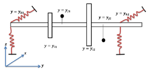
A complete model of rotor-bearing system with arbitrary conditions is shown in Figure 1.
In this model, the number of discs and their axial locations, the number and position of the bearings, the number of unbalance masses with different radius, magnitude, phase angle and their axial locations are completely arbitrary. In this model, the shaft is continuous and each bearing is modelled as two springs in horizontal and vertical directions.
Figure 1. A general model of the rotor-bearing system with arbitrary conditions
2.1 Energy terms
Consider a model of a rotor with an arbitrary number of discs, unbalance masses and bearings with arbitrary locations mounted on the continuous flexible shaft as shown in Figure 1. All energy terms of each of these parts are derived individually as follows:
One then easily shows that the vector of rotation of the disc is given by:
$\vec{\omega}_{R / R_{0}}=$$\left[\begin{array}{l}\omega_{x} \\ \omega_{y} \\ \omega_{z}\end{array}\right]=$$\left[\begin{array}{l}-\dot{\psi} \cos \theta \sin \phi+\dot{\theta} \cos \phi \\ \dot{\phi}+\dot{\psi} \sin \theta \\ \dot{\psi} \cos \theta \sin \phi+\dot{\theta} \sin \phi\end{array}\right]$ (1)
Let u and w be the coordinates of O in R0, the following coordinate y is constant. The mass of the disc given by MD and its tensor of inertia in O with x, y, z principal directions of inertia:
${{I}_{i0}}=\left[ \begin{matrix} {{I}_{Dx}} & 0 & 0 \\ 0 & {{I}_{Dy}} & 0 \\ 0 & 0 & {{I}_{Dz}} \\\end{matrix} \right]$ (2)
The kinetic energy of the disc is, in this case, given by:
${{T}_{D}}=\frac{1}{2}{{M}_{D}}\left( {{{\dot{u}}}^{^{2}}}+{{{\dot{w}}}^{^{2}}} \right)+\frac{1}{2}{{I}_{Dx}}\left( {{I}_{Dx}}{{\omega }_{x}}^{2}+{{I}_{Dy}}{{\omega }_{y}}^{2}+{{I}_{Dz}}{{\omega }_{z}}^{2} \right)$ (3)
where, ψ, θ and φ are the orientation angles of the coordinate system linked to the disc with respect to the fixed coordinate system (see Figure 3). The calculation of inertias and masses is detailed in the reference [20]. The expression of kinetic energy can be simplified. The angles and are small, the speed of rotation is constant (=) and the disk symmetrical (IDX = IDZ). In this case, the kinetic energy of the disc is given by the following relation:
${{T}_{D}}=\frac{1}{2}{{M}_{D}}\left( {{{\dot{u}}}^{^{2}}}+{{{\dot{w}}}^{^{2}}} \right)+\frac{1}{2}{{I}_{Dx}}\left( {{I}_{Dx}}{{\omega }_{x}}^{2}+{{I}_{Dy}}{{\omega }_{y}}^{2}+{{I}_{Dz}}{{\omega }_{z}}^{2} \right)$ (4)
The term IDY represents the gyroscopic effect (Coriolis). The term ½ IDY is constant and therefore has no influence in the equations.
$\frac{d}{dt}\left( \frac{\partial t}{\partial \dot{\delta }} \right)-\frac{\partial T}{\partial \delta }={{M}_{d}}\ddot{\delta }+{{C}_{d}}\dot{\delta }$ (5)
$\left[ {{M}_{d}} \right]=\left[ \begin{align} & \begin{matrix} {{k}_{xx}} & {} \\ 0 & {} \\\end{matrix}\begin{matrix} 0 & 0 \\ {{M}_{D}} & 0 \\\end{matrix}\begin{matrix} {} & 0 \\ {} & 0 \\\end{matrix} \\ & \begin{matrix} {{k}_{zx}} & {} \\ 0 & {} \\\end{matrix}\begin{matrix} 0 & {} \\ 0 & {} \\\end{matrix}\begin{matrix} {{I}_{Dx}} & 0 \\ 0 & {{I}_{Dz}} \\\end{matrix} \\\end{align} \right]$$\left[ {{C}_{d}} \right]=\Omega \left[ \begin{align} & \begin{matrix} 0 & {} \\ 0 & {} \\\end{matrix}\begin{matrix} 0 & 0 \\ 0 & 0 \\\end{matrix}\begin{matrix} {} & 0 \\ {} & 0 \\\end{matrix} \\ & \begin{matrix} 0 & {} \\ 0 & {} \\\end{matrix}\begin{matrix} 0 & 0 \\ 0 & {{I}_{Dy}} \\\end{matrix}\begin{matrix} -{{I}_{Dy}} & {} \\ 0 & {} \\\end{matrix} \\\end{align} \right]$
2.2 Kinetic energy of the shaft
The kinetic energy of the shaft can be written by extending the kinetic energy of a disk in longitudinal direction. Figure. 3 shows the reference frame of a disc mounted on flexible shaft. Then, it is possible to have.
${{T}_{s}}=\frac{\rho S}{2}\int_{0}^{L}{\left( {{{\dot{u}}}^{^{2}}}+{{{\dot{w}}}^{^{2}}} \right)dy}+\frac{\rho I}{2}\int_{0}^{L}{\left( {{{\dot{\psi }}}^{^{2}}}+{{{\dot{\theta }}}^{^{2}}} \right)dy}+\rho IL{{\Omega }^{^{2}}}+2\rho I\Omega \int_{0}^{L}{\dot{\psi }\theta dy}$ (6)
From the equations of the shaft, the disc and the bearings, the equation of motion of the rotor is written in the form:
$M\ddot{\delta }+C\left( \Omega \right)\delta +\dot{K}\delta =0$ (7)
Let us consider a rigid disc, represented in Figure 2, with the fixed and rotating reference marks respectively noted (X, Y, Z) and (x, y, z). The relationship between the two landmarks is established using Euler angles, in the form of three successive rotations as shown in Figure 2.
Figure 2. The disc and the fixed and rotating marks
Figure 3. Euler's angles
The aim of this research is to study the optimum stability by proper placement of different discs on the shaft. Optimization technique is used for a specific purpose. Analyzed enhanced disk positioning can help reduce rotor failure and verify higher stability certification.
In this work, two methods of system analysis, the Plackett-Burman statistical method, were combined to optimize the system properties, determine the most influencing factors and the finite element method to find out the gyroscopic effect on eigenvalues of rotor-bearing systems by Campbell. Graph, to fundamentally account for imbalance responses during the critical velocity passage. We designed a mathematical model under the name of rotor matrix in the software matlab that contains the geometry data of the rotor matrix element (tree data, disk data, and rotor matrix component geometry data.
In addition to stiffness and damping matrices as a set of nodes and elements to calculate values of imaginary and true frequency under 0-10000 rpm.
3.1 Rotor model "Rotor Lalanne"
A rotor dynamic system can be decomposed into subsystems. This allows for various detailed models components.
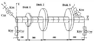
The used model is a rotor Lalanne with a length of 1.3m as shown in Figure 4. A mass of 115.66 kg is mounted on the shaft which is supported by two bearings respectively 0.2 (m) and 1.3 (m) apart from the left end. 5 stations are taken into consideration during harmonic analysis, in which the station numbers denote different nodes in the model: First bearing node (1), Disc (1), Disc (2), Disc (3), Second bearing (5). For the distributed rotor and the concentrated disc (1), the material density is 7800 kg / m3 and the modulus of elasticity is 2E11 N / m2. with a mass of 0.81 kg, disk (1) with a mass of 14.58 kg and disk (2) with a mass 45.95, disk (3) with a mass of 55.13 kg, polar inertia (0.123 0.976 1.171) kg.m2 and diametral inertia (0.0646 0.498 0.603) kg.m2.
Figure 4. Schematic model of the used model of rotor Lalanne
3.2 Calculation of real and imaginary system frequency values
Table 1. Rotor-bearing configuration data
|
Element Node No |
Node Location (cm) |
Bearing and Disk |
Inner Diameter (cm) |
Outer Diameter (cm) |
|
1 |
0.2 |
Bearing |
0 |
0.1 |
|
2 |
0.3 |
Disc |
0 |
0.1 |
|
3 |
0.5 |
Disc |
0 |
0.1 |
|
4 |
1 |
Disc |
0 |
0.1 |
|
5 |
1.3 |
Bearing |
0 |
0.1 |
A mathematical model was designed under the name of Rotor Lalanne using Matlab which includes the data of each element of the rotor kit (shaft, disc, and bearing), and also the stiffness and damping matrices in the form of a set of nodes and elements were used to determine the values of the stiffness and the real and imaginary frequency at a speed interval ranging from 0 to 10,000 rpm (Table 1).
4.1 Data of fluid film bearings
The response chosen is the imaginary frequency and the real frequency of a system rotor- bearings, calculated by Matlab software.
The factors examined in this study are:
- The diameters of the Lalanne d1, d2, d3.d4.
- Three disk positions p1, p2, p3.
- The shaft is mounted on two fluid film bearings where the stiffness (Kyy, Kzz) was determined using Matlab software.
- Kyz= Kyz = 0.
- Bearing 1: kyy1=7e7 (Ns / m), kzz1=6e7(Ns / m),
- Bearing 2: kyy2=5e7(Ns / m), kzz2=4e7(Ns / m),
- The components of damping are taken as:
Bearing 1: Cyy1 = 7e7 (Ns / m), Czz1=5e7(Ns / m),
Bearing 2: Cyy2 = 6e7 (Ns / m), Czz2=4e7(Ns / m).
4.2 Plackett-Burman
The experimental design methodology made it possible to generate a regression model. In this work we chose the Plackett-Burman plan. This choice is particularly driven by the required low cost: 20 trials must be counted. This number is low compared to a fully factor design, at two levels each A factor that requires 20 runs.
With regard to the selection of factors, we relied on the results of a two-level examination plan for each factor The Eleven factors studied and their field of study were grouped together in Table 2.
Table 2. The factors used in the study
|
factors |
Symbol |
Units |
Levels |
|
|
-1 |
1+ |
|||
|
The diameters |
d1=d2=d3=d4 |
(m)
|
0.05 |
0.15 |
|
Positions of the disc |
p1 p2 p3 |
(m) (m) (m) |
0.15 0.25 0.45 |
0.25 0.35 0.55 |
|
Stiffness Bearing 1 |
Kyy1 Kzz1 |
(Ns/ m) (Ns/ m) |
0 0 |
7e7 5e7 |
|
Stiffness Bearing 2 |
Kyy2 Kzz2 |
(Ns/ m) (Ns/ m) |
0 0 |
6e7 4e7 |
5.1 Response factors
The Plackett –Burman design is a very useful tool which enables to screen n variables using only n+ 1 experiment [21]. We use the Plackett-Burman (PBD) to improve rotor and determine the impact of discs position and the stiffness on rotary machine dynamics as well as knowing the diameters responsible for producing large effects on the frequency as well the reactions which increase or decrease the main effects.
PBD is a design experiment that works based on the first order polynomial model:
$y=\beta 0+\Sigma \beta \mathrm{i} X i$ (8)
where, y is the response, β0 is the model intercept, βi is the linear coefficient, and Xi is the level of the independent variable.
Therefore, this model only used to screen and evaluate the important variables that significantly influence the response and does not portray interaction among variables.
5.2 Analyze factorial design
The Plackett-Burman Plan allowed us to examine 11 factors (d1, d2, d3, d4, p1, p2, p3, kyy1, kyy2, kzz1, kzz2) in more detail to identify optimal conditions to determine the factors most influencing frequency. The results of this plan will be subject to the necessary statistical treatment. Table 3. It represents the fixing of factors at different levels.
Table 3. Plackett-Burman plan based on the experimental matrix
|
|
d1 |
d2 |
d3 |
d4 |
p1 |
p2 |
p3 |
kyy1 |
kyy2 |
kzz1 |
kzz2 |
FRQ img |
FRQreal |
|
1 |
0.05 |
0.15 |
0.15 |
0.05 |
0.15 |
0.25 |
0.45 |
7E+07 |
0 |
5E+07 |
0 |
114.35 |
692.14 |
|
2 |
0.15 |
0.15 |
0.15 |
0.15 |
0.15 |
0.25 |
0.55 |
7E+07 |
0 |
5E+07 |
4E+07 |
18.91 |
14.37 |
|
3 |
0.05 |
0.15 |
0.05 |
0.15 |
0.25 |
0.35 |
0.55 |
0 |
0 |
5E+07 |
4E+07 |
145.08 |
96.81 |
|
4 |
0.05 |
0.05 |
0.05 |
0.05 |
0.25 |
0.25 |
0.55 |
0 |
6E+07 |
5E+07 |
4E+07 |
32.11 |
15.85 |
|
5 |
0.05 |
0.05 |
0.05 |
0.15 |
0.15 |
0.35 |
0.45 |
7E+07 |
6E+07 |
5E+07 |
4E+07 |
35.38 |
0.75 |
|
6 |
0.15 |
0.15 |
0.05 |
0.05 |
0.25 |
0.35 |
0.45 |
7E+07 |
6E+07 |
0 |
0 |
31.56 |
45.1 |
|
7 |
0.15 |
0.05 |
0.05 |
0.05 |
0.15 |
0.35 |
0.45 |
7E+07 |
0 |
5E+07 |
4E+07 |
30.07 |
105.85 |
|
8 |
0.15 |
0.15 |
0.15 |
0.05 |
0.15 |
0.35 |
0.55 |
0 |
6E+07 |
5E+07 |
0 |
74.78 |
15.02 |
|
9 |
0.05 |
0.15 |
0.05 |
0.15 |
0.15 |
0.35 |
0.55 |
7E+07 |
6E+07 |
0 |
0 |
40.36 |
29.95 |
|
10 |
0.15 |
0.05 |
0.15 |
0.05 |
0.25 |
0.35 |
0.55 |
7E+07 |
0 |
0 |
4E+07 |
30.6 |
695.12 |
|
11 |
0.15 |
0.05 |
0.15 |
0.15 |
0.15 |
0.25 |
0.45 |
0 |
6E+07 |
0 |
4E+07 |
20.42 |
35.07 |
|
12 |
0.05 |
0.15 |
0.15 |
0.05 |
0.25 |
0.35 |
0.45 |
0 |
0 |
0 |
4E+07 |
0 |
36.38 |
|
13 |
0.05 |
0.05 |
0.05 |
0.05 |
0.15 |
0.25 |
0.45 |
0 |
0 |
0 |
0 |
0 |
70.57 |
|
14 |
0.05 |
0.15 |
0.15 |
0.15 |
0.25 |
0.25 |
0.45 |
7E+07 |
6E+07 |
0 |
4E+07 |
28.31 |
15.93 |
|
15 |
0.15 |
0.15 |
0.05 |
0.15 |
0.25 |
0.25 |
0.45 |
0 |
0 |
5E+07 |
0 |
16.16 |
20.88 |
|
16 |
0.15 |
0.05 |
0.15 |
0.15 |
0.25 |
0.35 |
0.45 |
0 |
6E+07 |
5E+07 |
0 |
13.2 |
31.34 |
|
17 |
0.05 |
0.05 |
0.15 |
0.05 |
0.25 |
0.25 |
0.55 |
7E+07 |
6E+07 |
5E+07 |
0 |
122.75 |
7.02 |
|
18 |
0.15 |
0.05 |
0.05 |
0.15 |
0.25 |
0.25 |
0.55 |
7E+07 |
0 |
0 |
0 |
8.41 |
17.3 |
|
19 |
0.05 |
0.05 |
0.15 |
0.15 |
0.15 |
0.35 |
0.55 |
0 |
0 |
0 |
0 |
0 |
126.3 |
|
20 |
0.15 |
0.15 |
0.05 |
0.05 |
0.15 |
0.25 |
0.55 |
0 |
6E+07 |
0 |
4E+07 |
66.72 |
16.77 |
6.1 Graphic representation of effects at Pareto chart
This diagram (Figure 5) makes it possible to extract the most important parameters. Among all the factors studied and at the chosen confidence level (α = 0.05), the strong factors (kzz1) and the position (p3) and diameter d2, appear to be very influential factors in the imaginary part frequency.
(a). Pareto chart
(b). Pareto plot of normalized
Figure 5. Pareto plot of normalized effects
Main effects diagram:
The main effects diagram tells us about the simultaneous influence of all factors on the frequency. We can from this diagram (Figure 6) conclude that the stiffness kzz1 and p3 and diameter d2, are the most influential factors positively on the imaginary part frequency.
Figure 6. Diagram of the main effects on frequency imaginary
6.2 Determination of significant effects and coefficients of the model
The effects values and the coefficients of regression of the model are given as bellow in Table 4.
Model Summary:
S R-sq R-sq (adj) R-sq (pred)
44.3783 53.23% 0.00% 0.00%
The polynomial regression equation for the primary model (before excluding the non-significant terms), is written as follows:
FRQ img = -96 - 208 d1 + 243 d + 17 d2 - 177 d3 + 27 p1 - 27 p2 + 250 p3 + 0.000000 kyy1+ 0.000000 kyy2 + 0.000001 kzz1 - 0.000000 kzz2.
The goal is therefore to find the optimal polynomial equation. Based on statistical analysis previous, by eliminating the quadratic terms and the two interactions d1, d2, d3, d4, p1, p2, p3, kyy1, kyy2, kzz1, kzz2 gets a new model with a good quality fit. These results are summarized in Table 5.
Table 4. Analysis of variance for imaginary frequency FRQ img
|
Term |
DF |
Adj SS |
Adj MS |
F-Value |
P-Value |
|
D1 |
1 |
2153 |
2153.2 |
1.09 |
0.326 |
|
D2 |
1 |
2959.5 |
2959.2 |
1.50 |
0.255 |
|
D3 |
1 |
15.3 |
15.26 |
0.01 |
0.932 |
|
D4 |
1 |
1561.3 |
1561.32 |
0.79 |
0.399 |
|
P1 |
1 |
37 |
36.96 |
0.02 |
0.894 |
|
P2 |
1 |
36.7 |
36.75 |
0.02 |
0.895 |
|
P3 |
1 |
3131.8 |
3131.75 |
1.59 |
0.243 |
|
Kyy1 |
1 |
425.3 |
425.32 |
0.22 |
0.655 |
|
Kyy2 |
1 |
520.3 |
520.30 |
0.26 |
0.621 |
|
Kzz1 |
1 |
7084.2 |
7084.22 |
3.60 |
0.094 |
|
Kzz2 |
1 |
9.8 |
9.76 |
0.00 |
0.946 |
Table 5. The used Runs in DOE
|
|
d1 |
d2 |
d3 |
d4 |
p1 |
p2 |
p3 |
kyy1 |
kyy2 |
kzz1 |
kzz2 |
FRQ img |
FRQreal |
|
1 |
0.05 |
0.05 |
0.05 |
0.15 |
0.15 |
0.35 |
0.55 |
7E+07 |
6E+07 |
0 |
4E+07 |
35.38 |
0.75 |
|
2 |
0.15 |
0.15 |
0.05 |
0.15 |
0.25 |
0.25 |
0.45 |
7E+07 |
0 |
5E+07 |
0 |
16.16 |
20.88 |
|
3 |
0.05 |
0.15 |
0.15 |
0.05 |
0.25 |
0.35 |
0.45 |
0 |
0 |
0 |
0 |
0 |
36.38 |
|
4 |
0.05 |
0.05 |
0.05 |
0.05 |
0.15 |
0.25 |
0.45 |
0 |
0 |
0 |
4E+07 |
0 |
70.57 |
|
5 |
0.05 |
0.15 |
0.15 |
0.15 |
0.25 |
0.25 |
0.45 |
7E+07 |
6E+07 |
5E+07 |
0 |
28.31 |
15.93 |
|
6 |
0.05 |
0.05 |
0.15 |
0.05 |
0.15 |
0.25 |
0.45 |
0 |
6E+07 |
5E+07 |
4E+07 |
18.91 |
14.37 |
|
7 |
0.05 |
0.15 |
0.15 |
0.15 |
0.15 |
0.35 |
0.55 |
7E+07 |
0 |
0 |
4E+07 |
0 |
126.3 |
|
8 |
0.15 |
0.15 |
0.05 |
0.05 |
0.15 |
0.25 |
0.55 |
0 |
0 |
5E+07 |
0 |
66.72 |
16.77 |
|
9 |
0.05 |
0.15 |
0.15 |
0.15 |
0.15 |
0.35 |
0.55 |
7E+07 |
6E+07 |
0 |
4E+07 |
40.36 |
29.95 |
|
10 |
0.15 |
0.15 |
0.05 |
0.05 |
0.25 |
0.25 |
0.55 |
7E+07 |
0 |
0 |
0 |
114.35 |
692.14 |
|
11 |
0.05 |
0.05 |
0.15 |
0.15 |
0.15 |
0.25 |
0.45 |
0 |
0 |
0 |
0 |
18.91 |
14.37 |
|
12 |
0.15 |
0.05 |
0.05 |
0.05 |
0.15 |
0.25 |
0.55 |
0 |
6E+07 |
5E+07 |
0 |
145.08 |
96.81 |
|
13 |
0.05 |
0.05 |
0.05 |
0.05 |
0.15 |
0.25 |
0.55 |
0 |
6E+07 |
5E+07 |
4E+07 |
32.11 |
15.85 |
|
14 |
0.15 |
0.05 |
0.15 |
0.15 |
0.25 |
0.35 |
0.55 |
7E+07 |
0 |
5E+07 |
4E+07 |
30.6 |
695.12 |
|
15 |
0.15 |
0.15 |
0.15 |
0.15 |
0.25 |
0.35 |
0.45 |
0 |
6E+07 |
0 |
4E+07 |
20.42 |
35.07 |
|
16 |
0.15 |
0.05 |
0.15 |
0.15 |
0.25 |
0.35 |
0.45 |
0 |
6E+07 |
5E+07 |
4E+07 |
13.2 |
31.34 |
|
17 |
0.15 |
0.05 |
0.05 |
0.15 |
0.25 |
0.25 |
0.55 |
7E+07 |
0 |
0 |
0 |
114.35 |
692.14 |
|
18 |
0.05 |
0.15 |
0.05 |
0.05 |
0.25 |
0.35 |
0.55 |
7E+07 |
6E+07 |
0 |
0 |
31.56 |
45.1 |
|
19 |
0.15 |
0.05 |
0.05 |
0.05 |
0.15 |
0.35 |
0.45 |
7E+07 |
0 |
5E+07 |
4E+07 |
30.07 |
105.85 |
|
20 |
0.15 |
0.15 |
0.15 |
0.05 |
0.25 |
0.35 |
0.45 |
0 |
6E+07 |
5E+07 |
0 |
74.78 |
15.02 |
S R-sq R-sq (adj) R-sq (pred)
13.7321 95.26% 88.74% 67.84%
We notice from Table 6, that all the parameters estimated for this model are significant. The optimal polynomial regression equation for the new model is written as following:
FRQ img = -10.8 + 709.8 d1 - 243.9 d4 + 316 d2 - 323.4 d3 - 231.6 p1- 290.6 p2+ 285.0 p3+ 0.000000 kyy1 + 0.000001 kyy2 - 0.000001 kzz1 - 0.000001 kzz2
The employed model incorporates both principal effects and two-way interaction. We employed the values of (P) to estimate the coefficients and effects. To find the main effects using α = 0.05, the principal effects of diameter values of d1 to kzz2 and their interactions which are statistically important; where their (P) values are lesser than 0.05.
Table 6. Regression coefficients estimated for imaginary frequency FRQ img after excluding non-significant terms (coded unit)
|
Term |
DF |
Adj SS |
Adj MS |
F-Value |
P-Value |
|
D1 |
1 |
10508 |
10508.1 |
55.72 |
0.000 |
|
D2 |
1 |
1710 |
1710.2 |
9.07 |
0.017 |
|
D3 |
1 |
1729 |
1728.9 |
9.17 |
0.016 |
|
D4 |
1 |
2309 |
2309.5 |
12.25 |
0.008 |
|
P1 |
1 |
1145 |
1145.3 |
6.07 |
0.039 |
|
P2 |
1 |
1909 |
1909.5 |
10.13 |
0.013 |
|
P3 |
1 |
2471 |
2470.5 |
13.10 |
0.007 |
|
Kyy1 |
1 |
1669 |
1669.2 |
8.85 |
0.018 |
|
Kyy2 |
1 |
4960 |
4959.8 |
26.30 |
0.001 |
|
Kzz1 |
1 |
2824 |
2824.2 |
14.98 |
0.005 |
|
Kzz2 |
1 |
3484 |
3483.7 |
18.47 |
0.003 |
Analysis of variance after excluding non-significant terms (Table 6), shows that all the terms are highly significant. We therefore conclude that the model improved is statistically better.
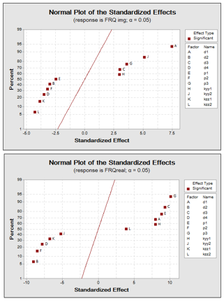
Diameter d1, stiffness kyy2, and position p3 are all important and have an effect on increasing the frequency of the imaginary part and this is shown in Figure 7.
The plot also states that:
The Diameter d1 has more effect on the frequency compared to stiffness kyy2 and position p3.
• Other diameters and other stiffness do not greatly affect the excitation frequency.
Figure 7. Representation of the standardized effects as an imaginary part
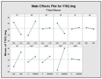
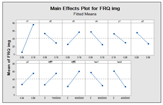
Then, the principal effect plots are sketched in MINITAB 17 as illustrated in Figures 8 and 9. The diameters effects, the stiffness, and the position of the discs on the excitation frequency show
Figure 8. Main effects plot for frequency- imaginary part
Figure 9. Main effects plot for frequency- real part
Figure 10. Interaction plot for imaginary frequency FRQ img and FRQ real
Interaction plots are typically used to visualize interactions during an ANOVA, in which the effect of one factor depends on the level of another factor. The diagram Figure 10 Shows that the parallel lines indicate the absence of interactions. The greater the difference in slope between the lines, the greater the degree of interaction.
The plot shows that interaction of p1 and kzz1 has greater difference in slope between lines. So, we can conclude that as p1 values vary from 0.15 to 0.25 the frequency decreases, while as kzz1 values increases from 0 to 5e7 the frequency increases.
Similarly, interactions (p1 and kyy2), (kyy1 and kyy2), (kyy1 and kzz1).
The plot shows that interaction of kzz1 and kzz2 has greater difference in slope between lines. So, we can conclude that as kzz1 values vary from 0 to 5e7 the frequency increases, while as kzz2 values increases from 0 to 4e7 the frequency decreases.
Similarly, interactions (p2 and kzz1), (p2 and kzz2) and versa for (d2 decreases, d4 increases).
The final step is to find the values of the factors that give the optimal answer. From the validated mathematical model and using the software, the 2D contours are produced graphically. These graphs make it possible to search for more desirable optimal solutions with the best possible precision. This allows us
To examine the results more clearly. The contour curves are generated using the MINITAB 17 software by the combination of the two induced factors. We have chosen each time one of the factors fixed at the 2 levels, high and low. The other two factors studied are represented on the X and Y axes. The value of the response is represented by a shaded region in the 2D contour curve. Figure 11 represents the 2D graphs which illustrate the evolution of the response according to the levels of the two factors.
Figure 11. Contour plots for imaginary frequency FRQ img and real frequency FRQ real
Through the Figure 11 when the position p1 values decrease, the frequency increases and are greater than 70, and when the stiffness kzz1 values change from 0 to 5e7 the frequency decreases, are less than 20.
Through the Figure 11 when the position p2 values increase, the frequency decreases and are less than 20, and when the stiffness kzz2 values change from 0 to 4e7 the frequency increases, are greater than 300.
Parameters:
|
Response |
Goal |
Lower |
Target |
Weight Upper |
Importance |
|
FRQ real |
Max |
0.75 |
695.12 |
1 |
1 |
|
FRQ img |
Max |
0.00 |
145.08 |
1 |
1 |
Solution1:
|
d1 |
d2 |
d3 |
d4 |
P1 |
P2 |
|
0.05 |
0.15 |
0.15 |
0.05 |
0.15 |
0.35 |
|
P3 |
Kyy1 |
Kyy2 |
Kzz1 |
Kzz2 |
FRQ Real FiT |
|
0.55 |
7e7 |
0 |
5e7 |
0 |
387.978 |
FRQ img Composite
Solution Fit Desirability
1 102.536 0.627801
Figure 12. Optimization plot "Solution 1"
Parameters:
|
Response |
Goal |
Lower |
Target |
Weight Upper |
Importance |
|
FRQreal |
Max |
0.75 |
695.12 |
1 |
1 |
|
FRQ img |
Max |
0.00 |
145.08 |
1 |
1 |
Solution2:
|
d1 |
d2 |
d3 |
d4 |
P1 |
P2 |
|
0.15 |
0.05 |
0.15 |
0.05 |
0.25 |
0.25 |
|
P3 |
Kyy1 |
Kyy2 |
Kzz1 |
Kzz2 |
FRQReal FiT |
|
0.55 |
7e7 |
0 |
0 |
0 |
1202.13 |
FRQ img Composite
Solution Fit Desirability
2 170.328 1
Figure 13. Optimization plot " Solution 2"
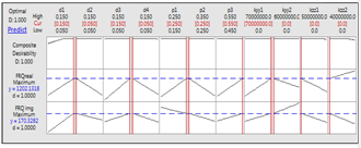
To find out how well the input variables met the objectives set for the answers. Individual desirability (d) shows how to optimize the settings for a single response. Composite desirability (D) evaluates how the settings optimize a set of responses overall. Desirability has a range from zero to one. One represents the ideal state. Zero indicates that one or more responses are outside its acceptable limits.
Figure 12, the composite Desirability (0.627801) is somewhat far from 1, which indicates that the settings did not achieve positive results for all responses as a whole compared to the results of the post-improvement, Figure 15 where the compound Desirability reached the value 1, which indicates that the factors whose values have changed achieved positive results and were more effective.
Obtain this desirability we would place the levels of factor at the values shown under the solution in red on the diagram Figure 13 (Table Solutions 2).
The rotor would be more stable if the disks were placed p3 and p2. Towards the ends of the rotor and the disc p1 towards the center of the rotor, and would be less stable if the discs p3 and p2 were placed towards the center of the rotor.
After determining the diameter d1 and stiffness coefficients Bearing kyy2 and p3 affecting the imaginary part of the excitation frequency, and the position p2 and diameter d3 are affecting the frequency of the real part, optimization plots are drawn based on the frequency values obtained from the matlab software (Figure14). The model of the rotor Lalanne is shown with different sections, discs and bearings.
In this part we use the finite element method for multi-disk rotor modeling because it provides clear modeling advantages, especially in measuring systems modeling as it provides physical damping in the column.
Figure 14. Rotor Lalanne with various sections
The rotational dissipation forces are proportional to the rotational speed and act tangentially over the rotor's orbit, and are known to cause instability after a certain rotational speed. A group of analyzes were found to determine the stability of the shaft system in terms of the stability limit of the rotational speed in addition to the response of the imbalance, which was summarized as follows:
1. Calculation of the undamped critical speeds
2. Evaluation of stability
3. Damped rotor mode shapes
4. Prediction of the rotor unbalance response
6.3 Calculation of the undamped critical speeds
Figure 15. Campbell diagram given by the calculation code
Figure 15 illustrates Campbell's diagram for the gyroscope system when internal damping is taken into account. The graph is drawn using the rotation frequencies (obtained from the imaginary part of the eigenvalues), and there are two positions: the first reverse rotation position "BW", where the rotor rotates in the opposite direction. The second position is "FW" rotation, where the rotor rotates in the direction of rotation. The critical speed corresponding to the first position and the critical speed corresponding to the second position are shown as follows:
The values of the first critical speeds:
|
Mode |
(Hz) |
(rpm) |
|
1 |
5.9356e+001 |
3.5613e+003 |
|
2 |
6.2683e+001 |
3.7610e+003 |
|
3 |
1.6090e+002 |
9.6539e+003 |
6.4 Evaluation of stability
The stability diagram (Figure 16) shows the evolution of the damping constants as a function of the speed of rotation. Since the real part is negative, the capacitance decomposes over time, so the rotor has a stable behavior, because the movement of the gyroscope tends to reduce the capacitance.
Figure 16. Stability diagram
6.5 Damped rotor mode shapes
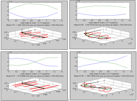
The mode shapes of a rotating shaft indicate the location of any point on the shaft during a whirling motion.
The first backward and forward movements of the simply supported rotor are traced using eigenvectors. Modes 2, 4 show the first form of three-dimensional mode for an un-damped rotor and modes 2, 4 show the same graph for a damped rotor (the internal damping indicating the starting point of the vortex).
In the reverse position, the back vortex rotates counter clockwise. The front vortex lines rotate clockwise. Figure 17 gives the relative deviation as a function of column length and confirms the results obtained in Table 7.
Table 7. shapes of the modes
|
Modes |
Precession |
Spin speed rpm |
|
1 |
invers |
FB =3563.1935 tr/min |
|
2 |
direct |
FW=3775.9718 tr/min |
|
3 |
invers |
FB=9773.8646 tr/min |
|
4 |
direct |
FW=10911.6638 tr/min |
Figure 17. Forms of modes and precession of forms of modes
Table 7 gives the result of the shapes of the modes, the initiative of the models and the speed of rotation of the patterns. Note that modes 1 and 3 are direct precession (the rotor rotates in the direction of rotation), and modes 2, 4 are invers precession (the rotor rotates in the opposite direction).
6.6 Prediction of the rotor unbalance response
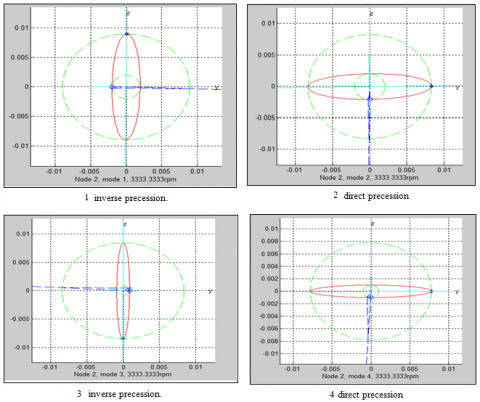
For the rotational speed 3333.3333 tr/ min, the orbits have a practically elliptical shape. The direction of precession of the orbits obtained is represented graphically in Figure 18 with the beginning of the orbit represented by a circle and the end represented by a star.
The figure shows that the orbits 4, 2 are described in the same direction as the speed of rotation of the rotor Ω. In this case, under the gyroscopic effects, the associated resonant frequency increases "direct precession".
The orbits 1, 3 are described in the opposite direction to the direction of the rotational speed of the rotor, which generates a softening effect and therefore a drop in the critical speed "inverse precession".
Figure 18. Orbits at 3333.3333 rpm
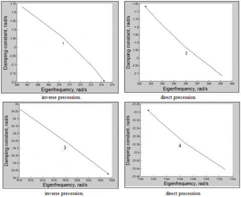
The root locus diagram (Figure 19) shows the evolution of the damping constant as a function of the natural frequency.
We notice, for example, that the direction of the modes, 1, 3, is from left to right (odd), the mode is therefore with inverse precession. On the other hand, the direction of modes 2, 4 is from right to left (even). The mode is with direct precession.
Figure 19. Root locus diagram
In this work we used as a preliminary step the Plackett-Burman screening design, carried out in order to select the factors most influencing the response. Among the various factors studied, diameters, position of the discs, the rigidity of the first bearings and the rigidity of the second bearings.
These factors are then examined by the response surfaces methodology using the Plackett-Burman design. To study the effect of the independent variables: the diameters, the positions of the discs, the rigidity of the system, we have modeled the response in the form of a polynomial according to these parameters. From the statistical study we can conclude that:
As a second step, the finite element method was used which aided in studying stability and identifying critical velocities, typical damping levels, and elliptical orbits. The results were obtained for different groups of disc positions to study the dynamic properties. Through the previous two methods, it was found that the rotor would be more stable if the disks were placed p3 and p2. Towards the ends of the rotor and the disc p1 towards the center of the rotor, and would be less stable if the discs p3 and p2 were placed toward the center of rotation. Thus, proper placement of disc can help reduce rotor failure and verify higher stability certification.
|
TD |
Kinetic energy of the disc |
|
IDY $\Omega $${{\psi }^{.}}$$\theta $ |
the gyroscopic effect (Coriolis) |
|
½ IDY $\Omega $2 |
constant |
|
TS |
Kinetic energy of the shaft |
|
Kyy1, Kzz1 |
stiffness coefficients Bearing 1 |
|
Kyy2, Kyy2 |
stiffness coefficients Bearing 2 |
|
Cyy1, Czz1 |
damping coefficients a gyroscopic effect Bearing 1 |
|
Cyy2, Czz2 |
damping coefficients a gyroscopic effect Bearing 1 |
|
DF |
Degrees of freedom from each source |
|
SS |
Sum of squares |
|
MS |
Mean squares |
|
F |
Calculate by dividing the factor MS by error |
|
P |
Use to determine whether a factor is signif. |
|
Secoff |
Standard error of the coefficient |
|
S |
Estimated standard deviation of the error |
|
Seq SS |
Sequential sum of squares |
|
Adj SS |
Adjusted sum of squares |
|
F |
The degrees of freedom for the test |
[1] http://www.itl.nist.gov/div898/handbook, accessed on 26 June 2006.
[2] Wass, J.A. (1997). Formal Experimental Design and Analysis for Immunochemical Product Development. Part I. IVD Technology Magazine 1997, September.
[3] Nijhuis, A., van der Knaap, H.C.M., Jond, S.D.E., Vandeginste, B.G.M. (1999). Strategy for ruggedness tests in chromatographic method validation. Anal. Chim. Acta, 391(2): 187-202. https://doi.org/10.1016/S0003-2670(99)00113-0
[4] Plackett, R.L., Burman, J.P. (1946). The design of optimum multifactorial experiments. Biometrika, 33(4): 305-325. https://doi.org/10.1093/biomet/33.4.305
[5] Yannis, L.L. (2001). A Plackett-Burnam screening design directs the efficient formulation of multicomponent DRV liposomes. J. Pharm. Biomed. Anal., 26(2): 255-263. https://doi.org/10.1016/S0731-7085(01)00419-8
[6] Trocine, L., Malone, C.L. (2000). Finding important independent variables through screening designs: Acomparison of methods. Proceedings of the Winter Simulation ConferenceJoines JA, Barton RR, Kang K, Fishwick PA, Eds, 749-754.
[7] Musznynska, M. (2005). Rotordynamics. CRC Press, Taylor & Francis Group, LLC, 1-30.
[8] Zorzi, E.S., Nelson, H.D. (1977). Finite element simulation of rotor-bearing systems with internal damping. ASME Journal of Engineering for Power, 99(1): 71-76. https://doi.org/10.1115/1.3446254
[9] Bhavikatti, S.S., Ramakrishnan, C.V. (1980). Optimum shape design of rotating disks. Computers and Structures, Pergamon Press Ltd, 11(5): 377-401. https://doi.org/10.1016/0045-7949(80)90105-4
[10] Chen, T.Y., Wang, B.P. (1993). Optimum design of rotor-bearing system with eigenvalues constraints. Journal of Engineering for Gas Turbines and Power, 115(2): 256-260. https://doi.org/10.1115/1.2906702
[11] Choi, B.G., Yang, B.S. (2000). Optimum shape design of rotor shaft using genetic algorithm. Journal of Vibration and Control, Sage Publication Inc., 6: 207-222 https://doi.org/10.1177/107754630000600203
[12] Shiau, T.N., Chang, J.R. (1993). Multi-objective optimization of rotor-bearing system with critical speed constraints. Journal of Engineering for Gas Turbine and Power, 115(2): 246-255. https://doi.org/10.1115/1.2906701
[13] Shabaneh, N.H., Zu, J.W. (2000). Dynamic analysis of rotor-shaft systems with viscoelastically supported bearings. Mechanism and Machine Theory, 35(9): 1313-1330. https://doi.org/10.1016/S0094-114X(99)00078-6
[14] Oncescu, F., Lakis, A.A., Ostiguy, G. (2001). Investigation of the stability and steady state response of asymmetric rotors, using finite element formulation. Journal of Sound and Vibration, 245(2): 303-328. https://doi.org/10.1006/jsvi.2001.3570
[15] Chasalevris, A.C. (2009). Vibration analysis of nonlinear- dynamic rotor-bearing systems and defect detection. PhD Dissertation, University of Patras, https://doi.org/10.13140/RG.2.1.4418.4727
[16] Xiang, J., Chen, D., Chen, X., He, Z. (2009). A novel wavelet-based finite element method for the analysis of rotor-bearing systems. Finite Elements in Analysis and Design, 45(12): 908-916. https://doi.org/10.1016/j.finel.2009.09.001
[17] Khanlo, H.M., Ghayour, M., Ziaei-Rad, S. (2011). Chaotic vibration analysis of rotating, flexible, continuous shaft-disc system with a rub-impact between the disc and the stator. Communications in Nonlinear Science and Numerical Simulation, 16(1): 566-582. https://doi.org/10.1016/j.cnsns.2010.04.011
[18] Mostefa, B., Kaddour, R., Mimoun, Y., Abdallah, N. (2018). Plackett-burman desing to study the influence of the stiffness of hydrodynamic bearings on the dynamic behaviour of turbo machinery. Mathematical Modelling of Engineering Problems, 5(4): 407-417. https://doi.org/10.18280/mmep.050418
[19] Naouri Abdallah Mostefa, B., Kaddour, R., Mimoun, Y. (2020). Investigate the effect of damping parameters of the hydrodynamic bearings using the optimization method of design of experiments. Mathematical Modelling of Engineering Problems, 7(1): 103-112. https://doi.org/10.18280/mmep.070113
[20] Sommerfeld, A. (1904). Zur hydrodynamischen theorie der schiermittelreibung. Z. angew. Math. Phys., 50: 97-155. https://doi.org/10.1002/zamm.19560360104
[21] Myers, R.H., Montgomery, D.C. (1995). Response Surface Methodology. Process and Product Optimization Using Designed Experiments. John Wiley&Sons, Inc., NY, USA.