Eduardo Chiarello | Juliana Almansa Malagoli*
© 2020 IIETA. This article is published by IIETA and is licensed under the CC BY 4.0 license (http://creativecommons.org/licenses/by/4.0/).
OPEN ACCESS
This paper aims to reduce the heating of the electromagnetic actuators of a magnetic bearing. The electrical current of the coils was above normal, so the need for a new coil design to reduce heating due to high currents. In this scenario, the proposed methodology allows minimizing copper losses using Particle Swarm Optimization, so that the best result of the design parameters will be used in the construction of the new coil for the actuator. For the development of this work, it was decided to use a computational tool for public use, FEMM (Finite Element Method Magnetics) to simulate the electromagnetic device. In the simulations, the densities of magnetic fluxes in the core and in the air gap are shown, as well as the energies, electromagnetic forces and losses in the copper of the electromagnetic actuator winding. Finally, an optimal model of the actuator is obtained through the use of optimization techniques. Therefore, the results obtained demonstrate that the proposed methodology is configured as an interesting strategy for the purpose of this work.
electromagnetic actuator, magnetic bearing, magnetic levitation, finite element method, particle swarm optimization
In various sectors of the industry (alternative energy sources, aerospace, automotive, etc.), more efficient equipment is sought, such as the case of Active Magnetic Bearings (AMBs) and Electromagnetic Actuators (EMAs). The main objective of the magnetic actuator is to generate forces and movement of the actuated device [1, 2]. These technologies allow rotating machines to operate close to their critical speeds. That is why it is important to study electromagnetic actuators.
Currently, the applications of electromagnetic actuators have been expanded to several areas mainly due to their high precision and the absence of physical contact between the shaft and the bearing, thus ruling out the use of lubricants between the parts and offering greater efficiency due to the absence of losses and friction [3-5]. Thus, enabling the actuators to be used in various areas. Among the applications of electromagnetic actuators that exploit this advantage, the following stand out:
• In turbo machinery (compressors and turbochargers), which allow the same factors to cause greater savings and a reduction in overall weight;
• In motors without mechanical bearings that allow a single control scheme for rotation and levitation and an increase in torque due to the absence of friction between the shaft and the bearing;
• In energy storage systems in flywheel systems, allowing high speeds to be achieved with low power losses;
• In biomedical, in cardiac pumps for people who need devices to keep their cardiac functions in full operation. The use of AMB avoids clotting problems for patients, as currently, conventional bearings can damage blood cells that are used as lubricants to avoid use and, therefore, contamination with the use of other lubricants;
• In turbo molecular pumps (devices used to create high vacuum for the manufacture of semiconductors) due to the absence of lubricants that can contaminate the process.
In recent years, several studies have proposed methodologies for electromagnetic actuators such as modelling of magnetic actuators on a bench with flexible suspended rotor [6] and active vibration control in flexible rotors using electromagnetic actuators [7]. Other applications are also mentioned, such as the optimization of the electromagnetic actuator [8] and the study and analysis of the electromagnetic actuator [9]. Finally, the characterization of an electromagnetic actuator applied to active vibration control in rotating machines was highlighted [10].
The hybrid bearing consists of four electromagnetic actuators, each control direction has two actuators. Electromagnetic actuators (EMA) apply only the forces of attraction and each actuator acts separately. Figure 1 shows a hybrid bearing with an electromagnetic actuator detail.
Figure 1. Hybrid bearing with detail of a studied electromagnetic actuator
This paper is a research project engaged in the design of electromagnetic actuators using optimization techniques and the finite element method. The initial phase of this paper is dedicated to the elaboration of the numerical computational model, to allow the analysis of the magnetic flux densities in the air gap and in the nucleus of the electromagnetic devices, in addition to the energy, force and losses in copper. Subsequently, the paper is dedicated to obtaining an optimum model of the actuator coil, through the use of optimization techniques. In this paper, particle swarm optimization will be used, for its easy implementation, it uses only mathematical operators and primitive structures without great computational cost.
The next sections of this article are organized as follows: in section 2, electromagnetic actuators are covered. Section 3 will write about the finite element method. Section 4 on particle swarm optimization. Section 5 deals with the methodology adopted in the development of this paper. Section 6 will present the results obtained. Finally, section 7 will describe the final considerations of this paper.
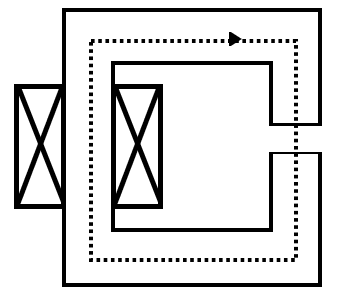
Magnetic circuits are characterized by containing one or more closed paths so that there is a passage of magnetic flux created by magnets or coils [3, 9]. Figure 2 shows a magnetic circuit with a closed path.
Figure 2. Magnetic circuit
To calculate the magnetic field, Ampere's Law is used, according to the following equations:
$\mathop{\oint }_{L\left( S \right)}^{{}}H.dl=NI$ (1)
$\mathop{\int }_{{{l}_{f}}}^{{}}{{H}_{f}}.dl+\mathop{\int }_{{{l}_{e}}}^{{}}{{H}_{e}}.dl=NI$ (2)
${{H}_{f}}{{l}_{f}}+{{H}_{e}}{{l}_{e}}=NI$ (3)
where, H is the magnetic field (A/m); N is the number of turns; I is the electric current (A); Hf is the magnetic field of the ferromagnetic core (A/m); He is the air gap magnetic field (A/m); lf is the average length in the ferromagnetic core (m); le is the average length in the air gap (m).
Eq. (1) associates the magnetic field and the average length of the materials that are part of the circuit, with the current that passes through the N wires around the core. The magnetic flux created by the coil passes through both the ferromagnetic core and the air gap in Figure 2. It is considered that there will be no losses in the circuit, so the flow through the air gap is the same as through the core [3, 11]. It is known that the flow is given by Eq. (4), the following development can be established:
$\Phi=\int_{S} \mathbf{B} \cdot d \mathbf{s}$ (4)
where, B is the magnetic flux density (T); ds is the area of a surface (m2).
Eqns. (5) and (6) establish the relationship between magnetic fields and permeability, straight sections of the air gap and the ferromagnetic core of the magnetic circuit.
$\Phi_{f}=\Phi_{e}$ (5)
${{\text{ }\!\!\mu\!\!\text{ }}_{\text{e}}}{{\text{H}}_{\text{e}}}{{\text{S}}_{\text{e}}}\text{=}{{\mu }_{0}}{{\text{H}}_{\text{f}}}{{\text{S}}_{\text{f}}}$ (6)
Reluctance expresses the difficulty of passing magnetic flux in a medium with permeability µr, length l and cross-section S, as well as Eq. (7).
${{\Re }_{i}}=\frac{l}{{{\text{ }\!\!\mu\!\!\text{ }}_{r}}S}$ (7)
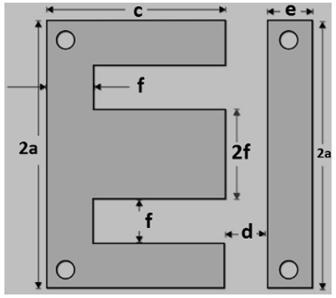
In addition, it is possible to define an actuator that is generally used to make forces on a rotor, so it is convenient to calculate the force exerted by an actuator, for this, the model in Figure 3 was used.
Figure 3. Model of an electromagnetic actuator
The reluctance of the ferromagnetic core was disregarded, as it is composed of a material with a high permissiveness µ. Thus, the reluctance is extremely low, to the point of being able to disregard it. With the air gap dimensions in Figure 3, the equivalent reluctance of the actuator can be obtained through the relationship between the reluctances of the three air gaps.
The association between the reluctances is shown in Eq. (8), with Ag being the cross-sectional area of the central air gap and d is the actuator air gap [11].
$R=\frac{2d}{{{\text{ }\!\!\mu\!\!\text{ }}_{\text{0}}}{{A}_{g}}}$ (8)
The inductance L is obtained from the number of turns N and the reluctance $\Re$ of the same, as in Eq. (9).
${{L}_{i}}=\frac{{{N}^{2}}}{\Re }$ (9)
Substituting Eq. (8) in Eq. (9), it is obtained:
$L=\frac{{{\text{ }\!\!\mu\!\!\text{ }}_{\text{0}}}{{A}_{g}}{{N}^{2}}}{2d}$ (10)
Eq. (10) determines the inductance of the actuator in Figure 3. With the inductance value it is possible to calculate the energy, as follows:
$W=\frac{L{{I}^{2}}}{2}$ (11)
Substituting Eq. (10) in Eq. (11), it is obtained:
$W=\frac{{{N}^{2}}{{I}^{2}}{{\text{ }\!\!\mu\!\!\text{ }}_{\text{0}}}{{A}_{g}}}{4d}$ (12)
Eq. (12) determines the energy in (J). The electromagnetic force is given by:
$F=\frac{{{N}^{2}}{{I}^{2}}{{\text{ }\!\!\mu\!\!\text{ }}_{\text{0}}}{{A}_{g}}}{4{{d}^{2}}}$ (13)
In the case of the actuator, the windings are considered as the resistive element, which in the presence of an electric current heats up. Thus, it represents a loss for the system.
Losses in copper are caused due to the Joule effect, through the transformation of electrical energy into thermal energy due to the passage of electrical current in a resistive element, causing its heating, where this energy dissipated in the form of heat is considered as a loss [3, 9, 11].
To calculate the electrical resistance of the actuator, the following equation will be used:
$R=\frac{{{\rho }_{copper}}.l}{{{A}_{wire}}}$ (14)
where, R is the electrical resistance of the winding (Ω); $\rho_{\text {copper}}$ is the resistivity of the copper conductor (1.72x10⁻⁸ Ωm); l is the length of the winding (m); Awire is the area of the conductor section (m2).
For the calculation of the conductor length, Eq. (15) is used.
${{L}_{e}}=2.N.b$ (15)
where, N is the number of turns; b is the depth of the electromagnetic actuator (m).
The area of a circle is calculated by the Eq. (16):
${{A}_{wire}}=\pi {{r}^{2}}$ (16)
where, r is the radius of the conductor (m).
To calculate the losses in copper, just calculate the resistive losses in the winding. To perform this calculation, Eq. (17) is used:
$P=R.{{I}^{2}}$ (17)
where, P is the loss in copper (W); I is the current that runs through the conductor (A).
The Finite Element Method (FEM) is a numerical procedure that aims to approximate the solution of complex problems, whose exact solution is given by partial differential equations (PDE) or ordinary (ODE) [11].
In addition, it consists of subdividing geometry into smaller elements, defined as finite elements, thus allowing complex problems to be divided into simpler problems. The exact solution is given by interpolating an approximate solution [12].
There are three steps to apply the FEM:
pre-processing;
processing;
post-processing.
The equations postulated by Maxwell from a group of differential equations that describe the physical behaviour of electromagnetic quantities, as well as different phenomena. Eqns. (18) and (19) are fundamental for magnetic modelling and are considered generalizations of Ampere's and Gauss's laws, respectively [13].
$rot~H=J+\frac{\partial D}{\partial t}$ (18)
$di{{v}_{{}}}B=0$ (19)
The magnitudes present in Maxwell's Eqns. (18) and (19) are the magnetic field H (A/m); magnetic induction B (T); the current surface density J (A/m2); electrical induction D (C/m2).
Eq. (18) shows that a magnetic field H can be created in two ways, either through a superficial density of current J or by a temporal variation of electrical induction D. Eq. (19) expresses that the magnetic flux that enters a volume is the same that comes out of it, that is, that the magnetic flux is conservative.
The magnetic field H is created when charges move in space, giving the notion of electric current that creates a vector field. The occurrence of an electric current in conductive materials occurs through the transit of electrons in the valence layer, called free electrons. These electrons move between vague positions of the atoms, making the final sum of charges to be zero, which makes the electric field almost zero [11, 12].
The multiplication of the magnetic permeability µ with the magnetic field at the same point is the name given for magnetic induction or magnetic flux density (T), as shown in Eq. (20).
$B=\mu H$ (20)
Magnetic permeability describes the degree of opposition of a material to the passage of a flow. Usually, the relative permeability of a substance is used with respect to air permeability, which is equivalent to 4π10-7 (H/m). The relative permeability is given by Eq. (21):
${{\mu }_{r}}=\frac{\mu }{{{\mu }_{0}}}$ (21)
Particle Swarm Optimization (PSO) is a method of optimizing non-linear functions, inspired by the behaviour of animals [14]. The population contains a set of particles, where each position that a particle occupies represents a possible solution to a given optimization problem.
In general, the PSO algorithm looks for the optimum, in the space of real numbers. For implementation, the steps that are presented below correspond to the canonical version of the algorithm [14, 15]. In 2001, according to Kennedy and Eberhart, the minimization of real functions through the most simplified technique is given by the proposal:
Eq. (22) updates the speed (vi) in each iteration (k) for each particle and Equation (23) updates the particle's position in the iteration [16, 17]:
$v_{\left( k+1 \right)}^{i}=wv_{k}^{i}+{{C}_{1}}{{r}_{1}}\left( pbest_{k}^{i}-x_{k}^{i} \right)+{{C}_{2}}{{r}_{2}}\left( gbest-x_{k}^{i} \right)$ (22)
$x_{\left( k+1 \right)}^{i}=x_{k}^{i}+v_{\left( k+1 \right)}^{i}$ (23)
where, $v_{(k+1)}^{i}$ is the updated particle speed; k+1 is the current time; k is the previous time; w is the algorithm's inertia constant; C1 is the individual acceleration coefficient responsible for controlling the distance of the movement of a particle in an iteration; C2 is the collective acceleration coefficient responsible for controlling the distance of the movement of a particle in an iteration; pbest is the best visited position of the particle; gbest is the best visited position among all particles; r1 and r2 are random numbers in the search space [0,1]; $x_{(k+1)}^{i}$ is the new position of the particle; $x_{k}^{i}$ is the previous position of the particle.
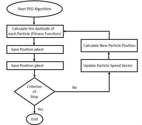
A basic flowchart of the PSO is illustrated in Figure 4.
Figure 4. Particle swarm algorithm flowchart
Therefore, as presented by Lobato et al. [16, 18], it is noted that the PSO comprises an extremely simple concept, since it only needs primitive mathematical operators for its implementation. This is advantageous because it generates a low-cost computational process, both in terms of memory and speed.
Throughout the discussion of results, we will focus on the analysis of the electromagnetic force, energy and losses in the copper of the electromagnetic actuator. In addition, magnetic flux densities were generated in the air gap and in the core. In this way, the actuator parameters are analysed in computer simulations. The procedures for validating the applied methodology are presented below:
The dimensions of the electromagnetic actuator and the modelling will be performed in the FEMM software;
In post-processing it is possible to analyse the magnetic flux densities in the different currents used from 0.9 to 3.6(A);
The analytical calculations of energy and electromagnetic force are compared with computer simulation;
The Particle Swarm Optimization was used, with the following criteria: number of iterations of 50, population size of 100, inertia factor of 1, individual acceleration coefficient of 1.5 and collective acceleration coefficient of 2.0;
Finally, losses are shown before and after the coil optimization.
In this paper, the silicon steel material is used in the core plates. Figure 5 shows the curve of the magnetic flux density versus the magnetic field of silicon steel. It is observed that the silicon steel saturates around 1.6 (T).
Section 6 shows in detail all the results analysed in this paper, such as: the electromagnetic force, the energy, the densities of magnetic fluxes in the core and air gap, and the losses in copper before and after the optimization of the electromagnetic device for the various electrical currents simulated.
Figure 5. BxH curve of silicon steel used in the actuator plate
This study considers Eq. (17) as the objective function (FO) of the studied problem. The objective function is to minimize losses in the copper of the electromagnetic actuator. Table 1 presents the variables, parameters and limits of the vector to minimize losses in the equipment's copper. The particle swarm optimization algorithm was used to analyse the optimal results.
Table 1. Variables, parameters and limits
|
Variables |
Parameters |
Minimum Limit |
Maximum Limit |
|
x(1) |
Electric current (A) |
0.92 |
5.25 |
|
x(2) |
Number of turns (windings) |
200 |
320 |
|
x(3) |
Air gap (mm) |
0.5 |
1.10 |
|
x(4) |
Wire diameter (mm) |
0.644 |
1.72 |
In addition, it was necessary to create restriction functions for the studied problem. The four functions can be highlighted:
$\text{g}\left( 1 \right)=\text{x}\left( 1 \right)-\text{x}\left( 3 \right)\ge 1$ (24)
$\text{g}\left( 2 \right)=4\text{*x}\left( 4 \right)-\text{x}\left( 1 \right)\ge 3$ (25)
$\text{g}\left( 3 \right)=2\text{*x}\left( 1 \right)-\frac{x\left( 4 \right)}{4}\ge 3$ (26)
$\text{g}\left( 4 \right)=4\text{*x}\left( 1 \right)+\text{x}\left( 2 \right)\ge 240$ (27)
After the optimization of the particle swarm optimization algorithm, the values of the parameters and the objective function were found. Table 2 shows the results of minimizing the loss in copper of the electromagnetic actuator.
Table 2. Parameter values after PSO algorithm execution
|
Parameters |
Optimum value |
|
x(1) = I |
1.6 |
|
x(2) = N |
230 |
|
x(3) = d |
0.64 |
|
x(4) = dia |
1.628 |
|
FO = P |
0.2438 |
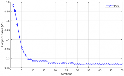
In general, the case study is very simple, with a mono-objective function and with restrictions. Figure 6 shows the copper loss profile obtained by the PSO Algorithm. The objective function is minimized, that is, the loss in copper is minimal.
It can be seen in Figure 6, that the optimization of the particle swarm optimization algorithm was able to obtain satisfactory results with rapid convergence to minimize the loss in the actuator in copper.
Table 3 shows the main parameters of the actuator before and after optimization obtained by using the Particle Swarm Optimization. The EMA silicon steel air gap measurements are represented in two dimensions by Figure 3 presented in section Electromagnetic Actuator.
Figure 6. Loss curve in the optimum copper of the electromagnetic actuator
Table 3. EMA parameters before and after optimization
|
Parameters |
Before |
After |
|
$\mu_{0}$ |
$4 \pi 10^{-7}$ |
$4 \pi 10^{-7}$ |
|
dia (wire diameter in mm) |
1.291 |
1.628 |
|
N (windings) |
228 |
230 |
|
a (mm) |
30 |
30 |
|
b (depth in mm) |
25 |
25 |
|
c (mm) |
40 |
40 |
|
d (mm) |
0.5 |
0.64 |
|
e (mm) |
10 |
10 |
|
f (mm) |
10 |
10 |
Table 4. Electromagnetic Force (N) before and after optimization
|
Current (A) |
Analytical Calculation Before Optimization |
Analytical Calculation After Optimization |
FEMM Simulation Before Optimization |
FEMM Simulation After Optimization |
|
0.9 |
26.44 |
16.4210 |
26.28 |
16.4649 |
|
1.8 |
105.77 |
65.6962 |
106.03 |
66.4645 |
|
2.7 |
237.98 |
147.8165 |
238.30 |
149.7470 |
|
3.6 |
432.09 |
262.7849 |
416.97 |
265.2760 |
Table 5. Energy (J) before and after optimization
|
Current (A) |
Analytical Calculation Before Optimization |
Analytical Calculation After Optimization |
FEMM Simulation Before Optimization |
FEMM Simulation After Optimization |
|
0.9 |
0.0132 |
0.0105 |
0.0135 |
0.0106 |
|
1.8 |
0.0528 |
0.0420 |
0.0546 |
0.0429 |
|
2.7 |
0.1189 |
0.0946 |
0.1218 |
0.0966 |
|
3.6 |
0.2115 |
0.1681 |
0.2124 |
0.1710 |
Table 6. Losses (W) before and after optimization
|
Current (A) |
Analytical Calculation Before Optimization |
Analytical Calculation After Optimization |
FEMM Simulation Before Optimization |
FEMM Simulation After Optimization |
|
0.9 |
0.12170 |
0.0710 |
0.12159 |
0.0771 |
|
1.8 |
0.48684 |
0.3078 |
0.48636 |
0.3086 |
|
2.7 |
1.09538 |
0.6926 |
1.09431 |
0.6943 |
|
3.6 |
1.94734 |
1.2313 |
1.94543 |
1.2343 |
Tables 4 and 5 show the values of electromagnetic forces and energy, respectively. In addition, it shows the numerical calculation obtained through Eqns. (12) and (13), respectively. Finally, the simulated value together with the variation of currents from 0.9 to 3.6 (A).
Table 6 shows the losses (W) in the actuator windings for currents from 0.9 to 3.6 (A). In addition, it shows the result of the numerical calculation obtained through Eq. (17) and the simulated value.
This way, it was found that the dimensions of the silicon steel core were not modified, but the diameter of the wire, the number of turns and the size of the air gap were changed. Thus, the winding resistance was reduced from 1,15Ω to 0,095Ω, consequently reducing the resistive losses in it, as shown in Table 6.
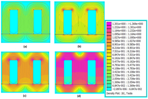
Figure 7 and Figure 8 shows the magnetic flux densities in the actuator core and air gap before and after optimization in currents 0.9 to 3.6 (A), respectively.
Figure 7. Magnetic Flux Densities before optimization: (a) 0.9(A); (b) 1.8(A); (c) 2.7(A); (d) 3.6(A)
Figure 8. Magnetic Flux Densities after optimization: (a) 0.9(A); (b) 1.8(A); (c) 2.7(A); (d) 3.6(A)
Note that after optimization there was a reduction in the values of electromagnetic force, energy of the actuator and losses in copper. For example, in the electric current of 1.8 (A) there was a reduction of 37.89%, 20.45% and 36.77%, respectively, of the strength, energy and loss in copper. Finally, the temperature reduction in the electromagnetic actuator stands out with the minimization of losses in copper. The next steps in this paper will be to maximize the electromagnetic force of the actuator and minimize losses in copper, in order to reduce the heating temperature of the device when it is connected to the magnetic bearing.
The present paper had the objective of reducing the heating in an electromagnetic actuator, using the particle swarm optimization algorithm. Using this optimization, new parameters for the coil and air gap were found, in this way, the losses in copper were considerably reduced, thus attesting to the effectiveness of the algorithm. It is also possible to observe a difference in relation to the results obtained before and after optimization, in the electromagnetic force and energy, due to the increase in the number of turns and the air gap of the actuator.
In the development of this paper, it was also found that the finite element method is fundamental for the characterization and understanding of electromagnetic actuators, due to the low percentage of errors between the theoretical results and the simulated results using the computational tool of public use FEMM (Finite Element Method Magnetics). The theoretical results were performed using a mathematical analysis of Maxwell's equations and the laws of material behaviour, making it possible to analyse electromagnetic forces, magnetic flux densities, energies and losses with variations in current and material values used in the core.
Therefore, it can be concluded that the particle swarm optimization method is consistent with reality, being an interesting strategy for reducing copper losses in electromagnetic actuators and consequently enabling the determination of the parameters of an actuator with great efficiency even in design phase.
The author Eduardo Chiarello thanks the “Fundação Araucária” for the resources destined to the development of this research paper. The authors are grateful for the infrastructure provided at the Energy System Laboratory of the Department of Electrical Engineering at the Federal University of Paraná.
|
H |
magnetic field, A/m |
|
N |
number of turns |
|
I |
electric current, A |
|
Hf |
magnetic field of the ferromagnetic core, A/m |
|
He |
air gap magnetic field, A/m |
|
lf |
average length in the ferromagnetic core, m |
|
le |
average length in the air gap, m |
|
B |
magnetic flux density, T |
|
ds |
area of a surface, m2 |
|
R |
electrical resistance of the winding, Ω |
|
L |
length of the winding, m |
|
Awire |
area of the conductor section, m2 |
|
b |
depth of the electromagnetic actuator, m |
|
r |
radius of the conductor, m |
|
P |
loss in copper, W |
|
$v_{(k+1)}^{i}$ |
updated particle speed |
|
k+1 |
current time |
|
k |
previous time |
|
w |
algorithm's inertia constant |
|
C1 |
individual acceleration coefficient responsible for controlling the distance of the movement of a particle in an iteration |
|
C2 |
collective acceleration coefficient responsible for controlling the distance of the movement of a particle in an iteration |
|
pbest |
best visited position of the particle |
|
gbest |
best visited position among all particles |
|
r1 and r2 |
random numbers in the search space [0,1] |
|
$x_{(k+1)}^{i}$ |
new position of the particle |
|
$x_{k}^{i}$ |
previous position of the particle |
|
Greek symbols |
|
|
$\rho_{\text {copper}}$ |
resistivity of the copper conductor (1.72x10⁻⁸ Ωm) |
|
$\mu_{0}$ |
relative air permeability (4π10-7 H/m) |
[1] Takei, K., Kitagawa, W., Takeshita, T., Fujimura, Y. (2019). Design and analysis of serial/parallel type of electromagnetic actuator. 19th International Symposium on Electromagnetic Fields in Mechatronics, Electrical and Electronic Engineering (ISEF), Nancy, France, pp. 1-2. https://doi.org/10.1109/ISEF45929.2019.9097031
[2] Kim, S., Lee, C., Choi, H. (2019). A study on electromagnetic-spring actuator for low cost miniature actuator systems. IEEE International Electric Machines & Drives Conference (IEMDC), San Diego, CA, USA, pp. 2008-2013. https://doi.org/10.1109/IEMDC.2019.8785169
[3] Waindok, A., Tomczuk, B., Koteras, D. (2019). Analysis of a novel permanent magnet electromagnetic valve actuator with FEM. 19th International Symposium on Electromagnetic Fields in Mechatronics, Electrical and Electronic Engineering (ISEF), Nancy, France, pp. 1-2. https://doi.org/10.1109/ISEF45929.2019.9096988
[4] Markovic, M., Jufer, M., Perriard, Y. (2008). Analytical force determination in an electromagnetic actuator. In IEEE Transactions on Magnetics, 44(9): 2181-2185. https://doi.org/10.1109/TMAG.2008.888573
[5] Noh, M.D., Gi, M.J., Kim, D., Park, Y., Lee, J., Kim, J. (2015). Modeling and validation of high-temperature electromagnetic actuator. In IEEE Transactions on Magnetics, 51(11): 1-4. https://doi.org/10.1109/TMAG.2015.2450364
[6] Oliveira, M.V.F., Silva, A.B., Silva, A.B., Koroish, E.H., Steffen, V. (2016). Modeling and characterization of a flexible rotor supported by AMB. In: De Clerck J., Epp D. (eds) Rotating Machinery, Hybrid Test Methods, Vibro-Acoustics & Laser Vibrometry, Volume 8. Conference Proceedings of the Society for Experimental Mechanics Series. Springer, Cham. https://doi.org/10.1007/978-3-319-30084-9_39
[7] Kim, Y.B., Hwang, W.G., Kee, C.D., Yi, H.B. (2001). Active vibration control of a suspension system using an electromagnetic damper. Proceedings of the Institution of Mechanical Engineers, Part D: Journal of Automobile Engineering, 865-873. https://doi.org/10.1243/0954407011528446
[8] Delinchant, B., Gruosso, G., Wurtz, F. (2009). Two levels modeling for the optimization of electromagnetic actuators. In IEEE Transactions on Magnetics, 45(3): 1724-1727. https://doi.org/10.1109/TMAG.2009.2012797
[9] Mateev, V., Terzova, A., Marinova, I. (2014). Design analysis of electromagnetic actuator with ferrofluid. 18th International Symposium on Electrical Apparatus and Technologies (SIELA), Bourgas, pp. 1-4. https://doi.org/10.1109/SIELA.2014.6871872
[10] Koroishi, E.H., Molina, F.A.L., Faria, A.W., Steffen Junior, V. (2015). Robust optimal control applied to a composite laminated beam. Journal of Aerospace Technology and Management, 7(1): 70-80. https://doi.org/10.5028/jatm.v7i1.389
[11] Luz, M.V.F., Dular, P., Leite, J.V., Kuo-Peng, P. (2014). Modeling of transformer core joints via a subproblem FEM and a homogenization technique. In IEEE Transactions on Magnetics, 50(2): 1009-1012. https://doi.org/10.1109/TMAG.2013.2284917
[12] Malagoli, J.A., Camacho, J.R., Luz, M.V.F., Ferreira, J.H.I., Sobrinho, A.M. (2015). Design of three-phase induction machine using differential evolution algorithm. In IEEE Latin America Transactions, 13(7): 2202-2208. https://doi.org/10.1109/TLA.2015.7273778
[13] Malagoli, J.A., Camacho, J.R. (2015). Automatic optimized design of a stator of induction motor using CAD Generator (Gmsh). In IEEE Latin America Transactions, 13(9): 2908-2914. https://doi.org/10.1109/TLA.2015.7350038
[14] Kennedy, J., Eberhart, R. (2001). Swarm Intelligence. Morgan Kaufmann Publishers.
[15] Lara, D.H., Cañizo, R.G.R., Cruz, E.A.M., Santiago, M.A.M. (2020). Optimal design of a drive shaft with composite materials through particle swarm optimization. in IEEE Latin America Transactions, 18(6): 1008-1016. https://doi.org/10.1109/TLA.2020.9099677
[16] Lobato, F.S., Machado, V.S., Steffen, V. (2016). Determination of an optimal control strategy for drug administration in tumor treatment using multi-objective optimization differential evolution. Computer Methods and Programs in Biomedicine, 131: 51-61. https://doi.org/10.1016/j.cmpb.2016.04.004
[17] Lostado, R., Roldán, P.V., Martinez, R.F., Mac Donald, B.J. (2016). Design and optimization of an electromagnetic servo braking system combining finite element analysis and weight-based multiobjective genetic algorithms. Journal of Mechanical Science and Technology, 30: 3591-3605. https://doi.org/10.1007/s12206-016-0720-6
[18] Yu, X., Li, B., Zhang, T., Tan, C., Yan, H. (2020). Variable weight coefficient optimization of gearshift actuator with direct driving automated transmission. in IEEE Access, 8: 4860-4869. https://doi.org/10.1109/ACCESS.2019.2963708