Design and Experimental Investigations on NOx Emission Control Using FOCDM (Fractional-Order-Based Coefficient Diagram Method)-PIλDµ Controller

Maheswari Chennippan* | Priyanka E. Bhaskaran | Thangavel Subramaniam | Balasubramaniam Meenakshipriya | Kasilingam Krishnamurthy | Varatharaj Arun Kumar
© 2020 IIETA. This article is published by IIETA and is licensed under the CC BY 4.0 license (http://creativecommons.org/licenses/by/4.0/).
OPEN ACCESS
This paper aims to explore experimental studies on the NOx removal process by using pilot plant packed column experimental hardware. Physical modeling based on chemical absorption equations is used to estimate the diameter concerning the height and L/G ratio. Hydrogen peroxide is used as the additive for achieving high NOx removal efficiency. The absorbent entering into the packed column has been controlled by varying its flow rate through the fractional order controller. The FOCDM-PIλDµ controller tuning parameters such as KP, τI, τD are determined using CDM (Coefficient Diagram Method) PID control strategy and the additional parameters of FOCDM-PIλDµ controller such as λ and µ are determined based on the PSO algorithm. The comparative analysis is performed with classical controllers like ZN-PID along with the CDM-PID controllers.
FOCDM-PIλDµ controller, PSO algorithm, CDM-PID controller, NOx emission control
In the industrial sectors concerned with fossil fuels, mining and the chemical processing industry, the major threats to human life are the emission of the Sulphur and nitrogen-based toxic content gases into the environment [1]. When these gases come into the atmosphere and get the oxidation process with the pure oxygen compounds it leads to the formation of oxides of nitrogen and Sulphur compounds causing acid rain and greenhouse effects to the surrounding circumstances [2, 3].
Its impact is not revealed directly, but it influences the Eco cycle in a rotating manner by harming the atmosphere frost which in turn exhibits its worst nature on human beings. The pioneering works were done by taking different categorization of combustion and reduction reaction by using different absorbent solutions to neutralize the Sulphur and nitrogen oxides compounds [4]. Each method gives its own merits and demerits to the human ecosystem and solving the rate is not efficient to the large-scale level. The later combustion methods seem to be cost higher and do not satisfy the regulatory standards. After analyzing various pre and post-treatment techniques with potassium permanganate can leads further to achieve the desired removal rate with minimal preparation standards [5]. The desulfurization process using flue gas as the main constituents methodology is the most effective technique to be implemented in many industrial problems to sort out the removing process of nitrogen compounds [6-9]. In the techniques, absorbents are considered as the solvent rather than the solid by pointing sodium chloride or hydrogen peroxide or potassium combined constituents [10-15].
The concentration of absorbent and the flue gas ratio is determined by the mathematical consideration based on the polluted gas entering as input. The regulation of the input and output are to be analyzed by utilizing the packed column structure for the emission control. Since the packed column reactor regulating properties can be most appropriate for the gas state analysis. When the oxidized gas gets reaction with the absorbent solvent, it separates the nitrogen oxide compounds as the single constituent atoms which get absorbed by the catalytic reaction which takes place at the terminal end of the column.
Mainly on enhancing the performance of the undertaken controller, the present work concentrating on the merits of both CDM control strategy in comparison with fractional calculus for NOx emission control. To evaluate the performance of the FOCDM-PIλDµ controller with classical tuning methods incorporated with PID structure through experimental analysis by using pure NOx gas over another consideration of mixed gas (SO2 with 4995 ppm +NO2 with 995 ppm concentration) as the input gas source to the chamber of the experimental investigation.
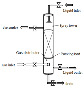
Figure 1. Packed column physical features
Based on the literature study, it is confirmed about the construction of the packed column should possess a very large mass transfer ratio which gives extreme NOx removal proficiency. The packed column capacity and its dimensions are determined based on physical modeling [16-24] and its structural schematic diagram is shown in Figure 1.
2.1 Mathematical modeling of the packed column
Determination of Lm/Gm ratio: To determine the flow rate of NOx (gas) and flow rate of liquid (H2O2) based on Henry's law formulated Eq. (1) is represented as:
$H=\frac{L_{m}}{G_{m}} *$ flowing factor (1)
where, Gm - Associated gas flow with molar rate and it is assumed as 0.0003383 kg/sec (1 m3/hr.), H - Henry’s constant is 0.0014 (Rolf Sander 1999), Lm - Liquid mass flow rate which is determined as 0.002285 kg/sec (5 lph), flooding factor (K4) is identified as K4 = 0.7 (Coulson & Richardson 1991).
Determination of packed column diameter: Packed column diameter is determined based on liquid and gas velocity. Diameter is optimized based on L/G ration pointing flooding factor around 72% is considered to attain the reasonable drop associated with the pressure parameter with maximum liquid and gas distribution. Sherwood correlation is used to find the flooding velocity requirement based on the calibration calculated flooding factor (K4) as 0.7 to be followed in the present work. Drop associated with the undertaken pressure (FLV) in the packed column is used to compute the packed column diameter. The pressure drop (FLV) is calculated based on Eq. (2).
$F_{l v}=\frac{L_{m}}{G_{m}} * \sqrt{\frac{P_{G}}{P_{L}}}$ (2)
Somewhere, ρG - vapor (NOx) mass (2.2809 kg/m3), ρL -liquid (HNO3) compactness (1490 kg/m3), Gm - Flow with respect to molar rate of NOx (0.0029972 kg/sec) and Lm - liquid flow with respect to molar rate (0.00166743 kg/sec).
Based on the above data and Eq. (2), pressure drop (FLV) is determined as 0.005994. The flooding factor needs to be considered while calculating the liquid flow rate into the column. With concern to the flooding factor, the corresponding flow rate of the gas/area computation in cross-sectional wise (Vw) is calculated based on Eq. (3),
$V_{W}=\left[\frac{K_{4}\left(P_{G}-P_{L}\right)}{1.31 F_{P}\left(\mu_{L} / \rho_{L}\right)^{0.1}}\right]$ (3)
where, ρG, ρL and K4 are taken from Eq. (1) and (2) then µL is the viscosity of the liquid and FP represents the packing factor (for the chosen 6mm into lax ceramic saddles, packing factor is 130). From the above data, Vw is calculated as 2.15 Kg/m2s.
The Area (A) on the packed column concerning the diameter (D) is determined from the Eq. (4).
$A=\frac{G_{m}}{V_{w}}$ (4)
where, Gm - Flow rate of the gas with molar percent 0.0003383 kg/sec (1 m3/hr.). Based on the Eq. (4), the area and diameter for fabricating the column with packed structures are estimated as 0.001573 m2 and 0.045 m.
Determination of packing height: The height of the packed column is utilized to examine the grasp uptime of the total liquid to be filled in the packed column. A packed bed increases the grasp up duration by increasing the accumulation of liquid volume which improves NOx removal proficiency. Calculation of packed column parameters like height (Z) of the column line is specified by the Eq. (5),
$Z=H_{o g} * N_{o g}$ (5)
where, NOG represents the total consumption of transfer units, HOG is the height associated with the transfer units. The total requirement of transfer units is estimated from the Eq. (6),
$N_{o g}=\ln \frac{l_{1}}{l_{2}}$ (6)
where, y1- NOx mole fraction entering into the packed column, y2 - NOx mole fraction leaving the packed column. The ratio of y1/y2 is determined as 5 then the number of a transfer unit (NOG) is determined as 1.6. The packed column is considered as discrete equipment instead it is continuous contact equipment so that the mass balance of the packed column can be determined. For many industrial applications, HOG is chosen between the ranges of 0.3 m to 1.2 m (Perry 1997). HOG is chosen as 0.3 m and hence by substituting the values of HOG and NOG, packed height Z is determined as 0.48 m. From these calculated parameters the packed column design has been determined and tabulated in Table 1.
Table 1. Parameters for designed packed column
|
S. No |
Parameter |
Calculated value |
|
1 |
Liquid flow rate |
5-10 lph |
|
2 |
Gas flow rate |
1 m3/hr. |
|
3 |
Packed column height |
0.70 m |
|
4 |
Packed column diameter |
0.045 m |
|
5 |
Packed area |
0.48 m |
|
6 |
Packing materials |
Intolax ceramic saddles with 6 mm diameter |
|
7 |
Absorbents |
NaClO2, H2O2, HNO3, and water |
|
8 |
Inlet concentration of NOX |
100 - 500 ppm |
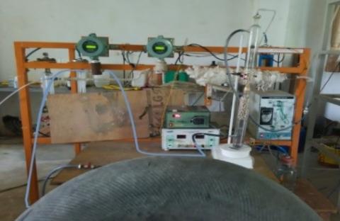
The experimental setup comprises of packed column with other accessories for the NOx removal process as shown in Figure 2. For experimentation, flue gas is taken from the IC engine exhaust emissions which comprise of different gases among those NOx plays a major concentration of above 500 ppm. This flue gas is supplied through the non-return check valve. NOx inlet gas sensor is fixed at this place for measuring inlet NOx concentration. The peristaltic pump holding the 0-5 lph flow rate is used for pumping the acid holding the H2O2 composition of 5 liters to pass into the packed column. H2O2 is given as an inlet liquid source from the top side of the packed column through the nozzle sprayer. To launch mass transformation between NOx and H2O2, the two states of gas and liquid are intermingled one another inside the column area.
Gas-liquid interaction exists due to the chemical contribution of NOx in the gas state starts to dissolve into hydrogen peroxide happening inside the packed column. The treated exhaust emission gas exists from the top end on the packed column structure. Absorption and composition of inlet an outlet NOx gas is measured using a NOx gas sensor and its equivalent digital data sent to the PC storage by interfacing with the data acquisition card. Based on the received of digital data, closed-loop control is enabled and the flow rate of the H2O2 is regulated.
Figure 2. A photographic view of the experimental setup for the NOX emission control process
3.1 Optimization of absorbents for NOX absorption
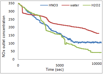
The experiments are conducted to optimize the absorbents for the NOx removal process. For these different absorbents are used such as water, H2O2, HNO3 is used and the results obtained are shown in Figure 3. While considering water as absorbent the removal efficiency obtained between 30 to 42%. During this reaction, the byproduct obtained is Nitric oxide (NO) as shown in Eq. (7) which is highly insoluble in water hence it is not considered for the present study.
$3 N O_{2}+H_{2} O \rightarrow H N O_{3}+N O$ (7)
During the reaction between NOx and HNO3, the removal efficiency is improved. By considering H2O2 (0.1 M) as absorbent, the passed hydrogen peroxide is oxidized by reacting with the flue gas mixture where it gets vaporized further to get dissolved with the formation of hydroxyl radicals. The formulated active OH radical starts to undergo an oxidation process to separate the NO and NO2 hence the removal efficiency is maintained above 90%. Hence H2O2 is considered an effective absorbent for further studies.
Figure 3. The response curve for different absorbents
3.2 Effect of H2O2 on NOX absorption
Though Hydrogen Peroxide (0.1 M) provides better removal efficiency, quite interesting results are found by regulating the H2O2 flow rate. H2O2 flow rate is sustained over the VDPID-03 Numerical controller. As shown in Figure 4, the flow rate between 0-5 lph is varied through the peristaltic pump and maintained for 10,000 sec until a steady-state response arrives.
Figure 4. The response curve for NOx outlet concentration at 100% DAQ opening
3.3 Model identification
Figure 4 shows that the flow rate of H2O2 influences the NOx removal efficiency in a better way. Figure 4 also ensures that the system is non-linear. The obtained transfer function to fall in First Order holding Time Delay (FOPTD) is undertaken for analysis in Eq. (8) [18].
$\mathrm{G}(\mathrm{s})=\frac{\mathrm{Kp}}{\tau \mathrm{pS}+1} e^{-\theta \mathrm{s}}$ (8)
For evaluating parameters from the transfer function, process gain (Kp) on the constrain of the time constant (τp) and time delay (ϴ) are examined using a two-point method. The identified FOPTD model of the process is represented as,
$G(s)=\frac{3.09}{11 S+1} e^{-2.14 s}$ (9)
The notation indications of Kp and τp represents process gain and time constant with a defined transport delay of ϴ (2.14 sec). The identified transfer function model is given in Eq. which is used as the transfer function for the NOx emission control process and it is used for controller studies [24].
This part of the paper reveals the control action provided by the implementation of classic controllers. The conformist controller tuning rules like Ziegler Nichols-PID along with Coefficient Diagram Method-PID techniques are implemented and its performances are analyzed. A tuning formula was proposed by Ziegler and Nichols in early 1942 expressed by Eq. (9) and its controller tuning rule is exposed in Table 2.
Figure 5. General block diagram of CDM-PID controller
Figure 6. Optimization of γ1 and γ2
Table 2. ZN-PID and CDM-PID tuning rules to attain respective gain for the controller structure
|
Controllers |
Parameters |
|||
|
Kc |
Τi(sec) |
Ki=(Kc/τi) |
Kd =(Kc*τd) |
|
|
ZN-PID |
1.7725 |
4.82 |
0.3677 |
0.8965 |
|
CDM-PID |
1.4916 |
20.49 |
0.0684 |
0.0223 |
4.1 CDM-PID controller design
It is a polynomial coefficient-based technique to obtain suitable and novel resolution for nonlinear systems that are represented as Coefficient Diagram Scheme (CDM) projected by Manabe [19]. The undertaken coefficient technique is an algebraic representation used to simplify the designing structure of the existing controller by considering the derived characteristic polynomial from the associated gain of the process and affords well-known results on the performance of the process by concentrating on the steadiness, response, and heftiness.
CDM-PID controller settings are computed for the NOx emission control process are given as follows and the polynomials are taken from the block diagram given above in Figure 5.
(1) The First-order transfer function model of the equation is given as:
$\mathrm{G}(\mathrm{s})=\frac{\mathrm{Kp}}{\tau \mathrm{pS}+1} e^{-\theta \mathrm{s}}=\frac{3.09}{11 \mathrm{~S}+1} e^{-2.14 \mathrm{~s}}$
(2) The FOPTD First order Pade’s approximation technique is used for FOPTD transfer function approximation as:
$G_{P}(S)=\frac{-7.4457 S+4.56}{2.66 S^{2}+24.46 S+2}$
The controller structure for CDM-PID is:
$G_{C}(S)=\frac{k_{2} S^{2}+k_{1} S+k_{0}}{l_{1} S}$
where, l1, k1, k2 and k0 represent controller polynomial coefficients.
(3) By combining steps 2 and 3 distinguishing polynomials are specified as,
$P(S)=A(S) D(S)+B(S) N(S)$
(4) The goal distinguishing polynomial is assumed as:
$P_{\text {target}}=a_{0}\left[\frac{\tau^{3}}{\gamma_{1} \gamma_{2}} S^{3}+\frac{\tau^{2}}{\gamma_{1}} S^{2}+\tau S+1\right]$
where, γ1 and γ2 are steadiness indices and τs - correspondent period constant.
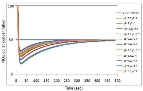
Here the γ1and γ2 values are to be optimized as per Manabe’s technique for determination of the coefficient of controller polynomials for achieving stability to the system. The optimization of gamma value is shown in Figure 6, such that g1 represents the γ1 and g2 represents γ2. From Figure 6, it is optimized that the values of γ1=3 and γ2=3.
(5) Like power, terms are equated as P(s) and Ptarget(s) then the controller polynomial coefficients (k2, k1, k0 and l1) are determined based on Manabe’s formula. k2 =11.5567, k1=12.7226, k0=1and l1=4.5562.
(6) The CDM based PID controller parameters in terms of CDM controller coefficients are computed by associating quantities of equivalent control relations of CDM controller
$u(t)=K_{p}\left(e(t)+\frac{1}{T_{i}} \int e(t) d t+\tau_{d} d(e(t)) / d t\right)=K_{P} e(t)+K_{i} \int e(t) d t+K_{d} d e(t) / d t$ (10)
By substituting the values in equation given in step 6, CDM-PID tuning constraints are attained as Kc=1.4916, TI=20.493min, TD=1.0517min. The determined parameters of ZN and CDM controller parameters are given in Table 3.
Based on the experimental model identification, the tuning parameters are computed for ZN-PID tuning in correspondence with the CDM-PID controller based on the Eq. (10). From the experimental results, the PID controller structure for enhancing the removal efficiency of the NOx emission control process and the system model is identified and developed using the MATLAB/SIMULINK platform. Performances of the controllers are analyzed using controller performance measures such as ISE, IAE, ITAE and ts. The readings are recorded for 10,000 to 14,000 sec until a steady-state condition is reached.
Table 3. Performance analysis of ZN and CDM-PID controllers on the set point of 20 ppm
|
Performance measures |
ZN-PID |
CDM-PID |
|
ISE |
346523.65 |
99910.79 |
|
IAE |
2019.376 |
415.8342 |
|
ITAE |
12540.5 |
628.22 |
|
Ts(sec) |
NIL |
8125 |
4.2 Performance analysis of ZN-PID and CDM-PID controller
From the computed tuning rule-based controller gain values, the experimental analysis is started with ZN-PID and CDM-PID controllers on the simulation platform using MATLAB.
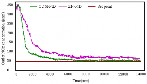
From Figure 7, reveals that the experimental curve of the CDM-PID controller influences the set point of 20 ppm at 8125 sec. The corresponding performance trial measures are revealed in Table 4, which ensures that the CDM-PID controller has fewer error indices (ISE, IAE and ITAE) than the ZN-PID controller.
Table 4. Performance evaluation analysis of ZN-PID and CDM-PID controllers at the setpoint of outlet NOx concentration of 50 ppm
|
Performance Measures |
ZN-PID |
CDM-PID |
|
ISE |
24286.72 |
19814.68 |
|
IAE |
3871.489 |
896.25 |
|
ITAE |
4985.027 |
734.223 |
|
ts (Sec) |
NIL |
7580 |
Figure 7. Efficiency graph of NOx emission control process using ZN and CDM-PID controllers
Also, the CDM controller settled at the set point of 20 ppm after 8125 sec whereas in the case of the ZN-PID controller almost 10 ppm offset is produced. These results confirm on the CDM-PID controller delivers enhanced performance than the ZN controller.
4.3 Robustness test of ZN-PID and CDM-PID controllers
Robustness tests are conducted at the set point of 50 ppm and its performances are recorded as shown in Figure 8 and Table 4.
From the results obtained from the robustness evaluation, the CDM-PID controller records improved presentation with the equivalent sceneries under various experimental operating circumstances. CDM-PID controller is forced to follow the set point at 7,580 sec as compared to the ZN-PID controller which produces 30 ppm offset. The error indices shown in Table 5 shows lesser values for the CDM-PID controller i.e. 44.7% reduced error in comparison with traditional benchmark-based ZN-PID controller.
Figure 8. Robustness test using CDM-PID and FOCDM-PIλDμ controller for the NOx removal process
Table 5. Performance measures of ZN comparing with CDM control calibration during load rejection analysis
|
Performance Measures |
ZN ̶ PID |
CDM ̶ PID |
|
ISE |
62589.01 |
19868.04 |
|
IAE |
4662.25 |
1025.82 |
|
ITAE |
6298.130 |
985.63 |
4.4 Load rejection analysis on ZN concerning CDM based controllers
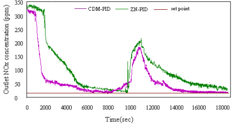
The third stage of the performance analysis is the load rejection test. These characteristics are used to analyze the performance of the controller when the external disturbance is added. For experimentation water is taken towards the flow of 0 to 1 lph is added as the disturbance into the mixing tank after 8000 sec under the working point of 20 ppm as exposed in Figure 9. Due to the external disturbance, NOx concentration increased up to 200 ppm, then by providing the controller action, NOx outlet concentration starts decreasing until it reaches the set point as shown in Figure 9.
Figure 9. Performance analysis of ZN comparing with CDM control structures at 20 ppm operating point during load rejection analysis
The performance measures with error indices are calculated for the period of 0 to 18000 sec with a step size of 5 sec, given in Table 5. From the experimental observation on the load rejection, it ensures that the implemented CDM-PID controller tries to follow the operating point on characterizing with the undertaken traditional ZN-PID controller. Thus, the CDM provides the enhanced performance, fractional Order built CDM-PIλDμ (FOCDM-PIλDμ) control strategy is imposed on the NOx emission control process.
PID strategy based on fractional order (FOPID) is a superior systematic design where its derivative and integral order are undertaken in integer format rather than fractional type. FOPID controller encompasses the fortitude of the important two significant constraints mainly as λ (fractional integral order) and μ (fractional derivative order) as evaluating with the traditional tuning approach of designing the PID structures. λ and μ are in fractions vary between 0 to 1, they upsurge the toughness of the arrangement and bounces an optimum plant control. The fractional-order tuning method is relying mainly on the standard CDM modification scheme for setting the tuning constraints Kc, KI and KD. λ and µ are optimized by the PSO tuning algorithm. Detailed basic equations for a fractional-order controller with the CDM PID controller is available in our previous research work.
5.1 Design steps for FOCDM-PIλDμ controller
FOCDM-PIλDμ Controller is premeditated by considering CDM strategy-based controller constraints (KP=0.3278, KI=0.0289, KD=0.096). The transfer function for the NOx emission control process is moving toward the fair optimum condition by utilizing first order oriented Pade approximation procedure,
$G_{p}(S)=\frac{-7.4457 S+4.56}{2.66 S^{2}+24.46 S+2}$
The fractional-order form of the controller transfer function is specified in the structure of:
$G_{P}(S) G_{C}(S)$$=\frac{-11.06 S^{3}-233 S^{2}+167.7 S+8.662}{478.9 S^{3}+501 S^{2}+49.92}$ (11)
By undertaking λ=1, μ=1 constraint, the bode plot is formulated in the open-loop to derive the transfer function is exposed in Figure 10. On the inferences on the bode plot, gain crossover frequency (ωu=0.796 rad/s) and calibrating frequency band towards the width of ([ωp, ωr]=[0.1ωt, 10 ωn]=[0.0796, 9.27] rad/sec) are evaluated.
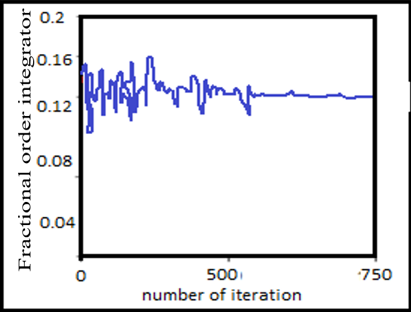
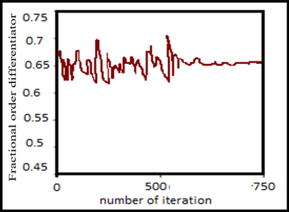
The Fractional-order integrator and differentiator values optimized to λ=0.1208 and μ=0.6929 from the convergence graph Figure 11.
Model representation of defined transfer function in an irrational form of FOCDM Controller is attained as:
$G_{c}(s)=1.499\left[1+\frac{1}{24.0987^{0.1247}}+0.0157^{2.309}\right]$ (12)
Estimated quantities of value integrator in the form of integral order (NI)=5 along with the differentiator range of (ND)=5 by involving the constraints with the term rate of y=1, λ=1.1208 and μ=1.6929. The obtained Eq. 10 is reformulated by considering only the rational term of function is exposed as:
$G_{c}(s)=0.335\left[1+\frac{1}{18.804 s^{\lambda}}+0.292 S^{\mu}\right]$ (13)
The Fractional order integrator and differentiator values optimized to λ=0.1208 and μ=0.6929. From the various analysis and calculation, the parameters of fractional order CDM-PID controller is determined as follows such as Kp=1.4016; KI=0.0684; KD=0.0223; λ=0.6929; μ=0.1208.
Based on the design detailed in section 5, the fractional-order CDM-PID controller parameters are determined. FOPID block in MATLAB/SIMULINK is used to interface real-time experimental hardware for closed-loop analysis. Three stages of performance analysis were to be done such as performance analysis, load rejection test and the robustness test.
6.1 First stage-performance analysis
Performance evaluation of the developed FOCDM-PIλDμ controller is validated in the scaled-down hardware established set up within the functional range of around 20 ppm and it is recorded as shown in Figure 12.
Figure 10. Bode plot Gp(s) on considering Gc(s) by fixing λ=1 and μ=1
Figure 11. Convergence graph for optimizing λ and μ
Figure 12. Operating evaluation of implemented FOCDM in comparison with CDM-PID controllers at a set range of 20 ppm
The performance and error analysis of the FOCDM-PIλDμ controller in comparison with CDM-PID is shown in Table 6. The performance quantities are recorded for the period of t=0 to 14,000 sec. The response of the FOCDM-PIλDμ controller attains the given range of targets at t=8095 sec and sustained. Then the response of the FOCDM-PIλDμ controller becomes stable whereas the CDM-PID controller produces little oscillations and it settles at t=12,000 sec with more ISE values.
Table 6. Evaluation of performance quantities of CDM-PID controllers at the set range of 20 ppm
|
Performance Measures |
CDM-PID |
FOCDM- PIλDμ |
|
ISE |
99910.79 |
67421.86 |
|
IAE |
415.8342 |
405.9685 |
|
ITAE |
628.22 |
206.3622 |
|
ts(sec) |
12000 |
8095 |
6.2 Second stage-robustness test
The second stage is the robustness test is attained from the investigational calibration is given in Figure 13 and the corresponding quantities of operation measures along with the error analysis are given in Table 7 at the set range of 50 ppm.
Figure 13. Performance of FOCDM in comparison with CDM controllers around investigation at 50 ppm
As compared to the CDM-PID controller, the FOCDM-PIλDμ controller furnishes robust comeback with a lesser range of ISE to the extent of 94.24% error minimization.
Table 7. Investigational quantities of FOCDM-PIλDμ in comparison with CDM-PID controllers of holding NOx outlet concentration in 50 ppm
|
Performance Quantities |
CDM-PID |
FOCDM -PIλDμ |
|
ISE |
19814.68 |
10420.98 |
|
IAE |
896.25 |
698.147 |
|
ITAE |
734.223 |
536.821 |
|
ts |
8280 |
7595 |
6.3 Third stage-load rejection test
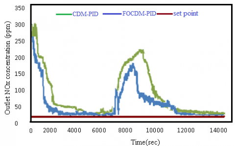
The load rejection properties of FOCDM-PIλDμ in comparison with undertaken CDM-PID controller are validated around the set range outlet maintenance of 20ppm NOx concentration. Step trouble is presented after 8000 sec onto the experimentation by way of allowing the water with the 0-1 lph flow rate as shown in Figure 14 and it demonstrates that both the traditional and implemented CDM-PID and FOCDM-PIλDμ controllers are established stability with the duration of 8500 sec.
Figure 14. Performance of FOCDM in comparison with undertaken CDM controller NOx at 20 ppm outlet concentration during load rejection analysis
After introducing the trouble, the NOx outlet concentration is improved to 240 ppm because the water is supplementary incorporated into the recirculation tank reduces the concentration of the H2O2. Initially, the concentration of NOx is increased towards the maximum value of 240 ppm and then it started to reduce gradually towards the setpoint due to controller action.
After 12,000 sec, NOx concentration is following to the equivalent functioning point due to the controller trigger feedback activation. On observation, the clear inference is FOCDM-PIλDμ controller damps the annoying the input variations and its better experimental acceleration is also confirmed by the performance quantities as exposed in Table 8.
Table 8. Performance measures of FOCDM and CDM controllers at 20 ppm operating point
|
Performance Measures |
CDM-PID |
FOCDM- PIλDμ |
|
ISE |
19868.04 |
10502.273 |
|
IAE |
1025.82 |
943.25 |
|
ITAE |
985.63 |
648.829 |
This paper has been undertaken to develop a simple and robust control strategy for the NOx emission control process. The experimental set up accomplishes a packed column along with the effective packing material combination that is optimized through mathematical modeling. Based on the mathematical modeling various parameters such as packed column holding the diameter (50 mm), column around the height (700 mm), packing height of the interfacial area (400 mm), minimum inlet liquid flow rate (3 lph) are determined. 0.1 M concentration of H2O2 is considered as an absorbent through various experimental works that give better high removal efficiency. Enhanced controller performance is indispensable to normalize the absorbent H2O2 flow rate to improve NOx removal efficiency. To normalize the H2O2 flow rate, CDM-PID design incorporating fractional order controller is intended by combining the concepts of fractional calculus and Coefficient Diagram Method (CDM). Initially, the classical controllers on pointing ZN-PID along with CDM-PID controllers are considered and the performance analysis was done. The tuning parameters of FOCDM-PIλDµ controller such as KP, TI, and TD were determined based on CDM design strategy (Kc =1.4016; TI=20.4938 min; TD=0.0517min).
The optimal ranges of λ and μ were calculated based on the PSO optimization technique. The computed parameters of FOCDM-PIλDμ controller were Kc =1.4016; Ti=20.4938 min; TD=0.0517 min; λ=0.6929; μ=0.1208. The supplementary tuning quantities λ and μ associated with the fractional order controller is used essentially for dropping the settling time in association with the errors. The FOCDM-PIλDμ controller tuning quantities terms λ and μ are calibrated with fraction form to enhance the robustness of the emission control process and affords the most approving control on the validating closed-loop system. Implementation of a packed column with a controller efficiently reduces the diesel engine exhaust containing NOx gas. Hence this experimental setup and the control action will also provide the necessary control action in the industrial environment.
The recommendations for further research are pinpointed as:
|
N(s) |
Numerator polynomial concerned with transfer function |
|
D(s) |
Denominator polynomials concerned with transfer function |
|
A(s) |
Polynomial corresponding to the forward denominator concerned with transfer function |
|
F(s) |
Polynomial corresponding to the Reference numerator concerned with transfer function |
|
B(s) |
Polynomial corresponding to the Feedback numerator concerned with transfer function |
|
P(s) |
Closed-loop system pointing characteristic polynomial |
|
Ptarget(s) |
Closed-loop system pointing target polynomial |
|
li, ki and ai |
Coefficients of CDM controller polynomials |
|
C(s) |
Main controller |
|
Cf(s) |
Feed forward based controller |
|
k1 and k0 |
Parameters associated with CDM tuning rule |
|
Kc and Ti |
Parameters associated with CDM-PI tuning rule |
|
SO2 |
Sulphur dioxide |
|
H2O2 |
Hydrogen peroxide |
|
H2SO4 |
Sulphuric acid |
|
Kp |
Process gain |
|
tr |
Rise time |
|
ts |
Settling time |
|
%Mp |
Peak overshoot |
[1] Magrini, A., Lazzari, S., Marenco, L., Guazzi, G. (2017). A procedure to evaluate the most suitable integrated solutions for increasing energy performance of the building’s envelope, avoiding moisture problems. International Journal of Heat and Technology, 35(4): 689-699. https://doi.org/10.18280/ijht.350401
[2] Giernacki, W., Sadalla, T., Gośliński, J., Kozierski, P., Coelho, J.P., Sladić, S. (2017). Rotational speed control of multirotor UAV's propulsion unit based on fractional-order PI controller. In 2017 22nd International Conference on Methods and Models in Automation and Robotics (MMAR), IEEE, pp. 993-998. https://doi.org/10.1109/MMAR.2017.8046965
[3] Donuk, K., Özbey, N., İnan, M., Yeroğlu, C., Hanbay, D. (2018). Investigation of PIDA Controller Parameters via PSO Algorithm. In 2018 International Conference on Artificial Intelligence and Data Processing (IDAP), pp. 1-6. https://doi.org/10.1109/IDAP.2018.8620871
[4] Maheswari, C., Priyanka, E.B., Meenakshipriya, B. (2017). Fractional-order PIλDµ controller tuned by coefficient diagram method and particle swarm optimization algorithms for SO2 emission control process. Proc IMechE, Part I: J Systems and Control Engineering, 231(8): 587-599. https://doi.org/10.1177/0959651817711626
[5] Priyanka, E.B., Maheswari, C., Thangavel, S. (2018). Remote monitoring and control of an oil pipeline transportation system using a Fuzzy-PID controller. Flow Measurement and Instrumentation, 62: 144-151. https://doi.org/10.1016/j.flowmeasinst.2018.02.010
[6] Priyanka, E., Maheswari, C., Thangavel, S. (2019). Remote monitoring and control of LQR-PI controller parameters for an oil pipeline transport system. Proceedings of the Institution of Mechanical Engineers, Part I: Journal of Systems and Control Engineering, 233(6): 597-608. https://doi.org/10.1177/0959651818803183
[7] Priyanka, E., Maheswari, C., Ponnibala, M., Thangavel, S. (2019). SCADA based remote monitoring and control of pressure & flow in fluid transport system using IMC-PID controller. Advances in Systems Science and Applications, 19(3): 140-162. https://doi.org/10.25728/assa.2019.19.3.676
[8] Priyanka, E.B., Maheswari, C., Thangavel, S. (2018). Proactive decision making based IoT framework for an oil pipeline transportation system. In International Conference on Computer Networks, Big data and IoT, Springer, pp. 108-119. https://doi.org/10.1007/978-3-030-24643-3_12
[9] Priyanka, E.B., Maheswari, C., Thangavel, S. (2018). IoT based field parameters monitoring and control in press shop assembly. Internet of Things, 3-4: 1-11. https://doi.org/10.1016/j.iot.2018.09.004
[10] Priyanka, E.B., Maheswari, C., Thangavel, S., Bala, M.P. (2020). Integrating IoT with LQR-PID controller for online surveillance and control of flow and pressure in fluid transportation system. Journal of Industrial Information Integration, 17: 100127. https://doi.org/10.1016/j.jii.2020.100127
[11] Subramaniam, T., Bhaskaran, P. (2019). Local intelligence for remote surveillance and control of flow in fluid transportation system. Advances in Modelling and Analysis C, 74(1): 15-21. https://doi.org/10.18280/ama_c.740102
[12] Priyanka, E.B., Krishnamurthy, K., Maheswari, C. (2016). Remote monitoring and control of pressure and flow in oil pipelines transport system using PLC based controller. In 2016 Online International Conference on Green Engineering and Technologies (IC-GET), IEEE, pp. 1-6. https://doi.org/10.1109/GET.2016.7916754
[13] Priyanka, E.B., Maheswari, C., Thangavel, S. (2020). A smart‐integrated IoT module for intelligent transportation in oil industry. International Journal of Numerical Modelling: Electronic Networks, Devices and Fields, e2731. https://doi.org/10.1002/jnm.2731
[14] Maheswari, C., Priyanka, E.B., Thangavel, S., Ram Vignesh, S.V., Poongodi, C. (2020). Multiple regression analysis for the prediction of extraction efficiency in mining industry with industrial IoT. Production Engineering, 14: 457-471. https://doi.org/10.1007/s11740-020-00970-z
[15] Bhaskaran, P.E., Chennippan, M., Subramaniam, T. (2020). Future prediction & estimation of faults occurrences in oil pipelines by using data clustering with time series forecasting. Journal of Loss Prevention in the Process Industries, 66: 104203. https://doi.org/10.1016/j.jlp.2020.104203
[16] Priyanka, E.B., Thangavel, S., Pratheep, V.G. (2020). Enhanced digital synthesized phase locked loop with high frequency compensation and clock generation. Sensing and Imaging, 21(1): 1-12. https://doi.org/10.1007/s11220-020-00308-0
[17] Priyanka, E.B., Thangavel, S., Venkatesa Prabu, D. (2020). Fundamentals of wireless sensor networks using machine learning approaches: Advancement in big data analysis using Hadoop for oil pipeline system with scheduling algorithm. Deep Learning Strategies for Security Enhancement in Wireless Sensor Networks. IGI Global, 233-254. https://doi.org/10.4018/978-1-7998-5068-7.ch012
[18] Priyanka, E.B., Thangavel, S., Madhuvishal, V., Tharun, S., Raagul, K.V., Shiv Krishnan, C.S. (2020). Application of integrated IoT framework to water pipeline transportation system in smart cities. In Intelligence in Big Data Technologies-Beyond the Hype, pp. 571-579. https://doi.org/10.1007/978-981-15-5285-4_57
[19] Priyanka, E.B., Subramaniam, T. (2018). Fuzzy logic forge filter weave pattern recognition analysis on fabric texture. International Journal of Electrical and Electronic Science, 5(3): 63-70.
[20] Priyanka, E.B., Thangavel, S. (2018). Optimization of large-scale solar hot water system using non-traditional optimization technique. Journal of Environmental Science and Allied Research, 2018(2): 43-52.
[21] Kao, C.C., Chuang, C.W., Fung, R.F. (2006). The self-tuning PID control in a slider–crank mechanism system by applying particle swarm optimization approach. Mechatronics, 16(8): 513-522. https://doi.org/10.1016/j.mechatronics.2006.03.007
[22] Chen, Y.J., Wu, Q.H. (2011). Design of PID controller based on PSO algorithm and FPGA. In 2011 2nd International Conference on Intelligent Control and Information Processing, IEEE, Harbin, China, 2: 1102-1105. https://doi.org/10.1109/ICICIP.2011.6008424
[23] Das, S., Pan, I., Das, S., Gupta, A. (2012). A novel fractional order fuzzy PID controller and its optimal time domain tuning based on integral performance indices. Engineering Applications of Artificial Intelligence, 25(2): 430-442. https://doi.org/10.1016/j.engappai.2011.10.004
[24] Zeng, G.Q., Chen, J., Dai, Y.X., Li, L.M., Zheng, C.W., Chen, M.R. (2015). Design of fractional order PID controller for automatic regulator voltage system based on multi-objective extremal optimization. Neurocomputing, 160: 173-184. https://doi.org/10.1016/j.neucom.2015.02.051