Anil Kumar Yadav* | Pawan Kumar Pathak | Prerna Gaur
© 2020 IIETA. This article is published by IIETA and is licensed under the CC BY 4.0 license (http://creativecommons.org/licenses/by/4.0/).
OPEN ACCESS
The objective of this paper is to design three different robust controllers such as proportional-integral (PI), internal model control (IMC), and H∞ control techniques for position control of the computerized numeric controlled machine tool (CNCMT) system. The proposed controllers aim to control the servo motor that regulates the position of the machine table and also enhances the robustness of the CNCMT system under the influence of parametric uncertainties. The stability of the uncertain CNCMT system with all designed controllers is investigated using Kharitonov’s theorem. The stability margin (SM) criterion is utilized for robustness analysis.
CNC machine tool, IMC, Kharitonov’s theorem, H∞ controls theory, robustness analysis
A computerized numeric controlled (CNC) machine is a highly integrated mechatronic system and it was developed to control the motion and operation of machine tools [1]. The CNCMT system is used mainly for drilling, cutting, milling, boring, finishing, welding, and aligning operations in automotive, aerospace, electrical, and instrumentation industries [2, 3]. In the CNCMT system, the information related to the structure of the workpiece is stored in the computer in the form of 'm-code'. The disturbances occurring during the machining process should be minimized to achieve high precision and operational efficiency [4-6]. The structured or parametric and unstructured uncertainties are presented in all practical control systems [7]. The source of parametric uncertainty in the CNCMT system is deficient in clear-cut knowledge of parameters, and few parameters like inertia and friction and varied under running conditions, therefore the system is called the uncertain CNCMT system. Hence the robustness analysis of the CNCMT system is essential and as proposed in this paper. To accomplish the most wanted position of machine table alongside the external disturbances and the parametric uncertainty three different robust controllers such as PI, IMC, and H∞ controllers are presented. Due to the presence of the derivative 'D' term in the PID controller, a derivative kick occurs and as a result, the controller output becomes dangerously high which may damage the actuator, in the present case, a servomotor. An integral 'I' control, a steady-state error is nullified but overshoot (OS) reaches to very high magnitude. Therefore, a PI type controller is used for position control of uncertain CNCMT system.
Indeed, the design of a low order controller is often more difficult than the design of a high order complex controller [8]. A robust PI controller is designed using Kharitonov’s theorem with the worst gain margin (GM) and phase margin (PM) because it plays an important role concerning the robustness of the system [9, 10]. In 1978, Kharitonov published his work in form of a research paper in a journal which is well taken for robust control problem [11]. So far, Kharitonov's theorem has been applied to various engineering applications such as mechanical systems [12], vehicle system [13], and an electrical system like DC-DC converter [14], load frequency control [15], and permanent magnet synchronous motor [9]. IMC policy was developed by Garcia and Morari [16], the design strategy of IMC is broadly documented that can realize the robust performance for tracking and disturbance rejection from the system response [17, 18]. The industrial applications of IMC for an electro-mechanical system such as heavy-duty vehicles [17, 19, 20], power system [21], and milling CNCMT system [22] are discussed. The robust H∞ controller using mixed sensitivity approach addresses the problem of system robustness by designing controllers in presence of noise and disturbance in the system [23, 24]. The method of selecting weighting functions for H∞ control has been discussed by Tewari et al. [25-27]. The various applications of the H∞ control theory is presented by Yadav et al. [13, 25, 26]. The modern and artificial intelligence-based control techniques such as fuzzy logic, adaptive, and artificial neural network-based controls of CNCMT is presented in the papers [1, 2, 22, 28, 29]. The benefits of artificial intelligence-based techniques such as fuzzy logic and artificial neural network are to reduce the mathematical complexity of controller design for the actual nonlinear, time-varying, and uncertain systems.
The effects of parametric uncertainty and disturbance on uncertain CNCMT systems with all three designed controllers are analyzed as proposed in this paper. The performance specifications such as OS, settling time (ST) and rise time (RT), and SM are considered for performance analysis of uncertain CNCMT system with designed controllers. A comparative performance analysis of controllers for the CNCMT system is presented to identify the superior controller over all the controllers designed in this paper. The robustness of the CNCMT system against parametric uncertainty using all designed controller is measured in terms of SM. Apart from OS, RT, ST, and SM performance parameters, the input disturbance and sensor noise rejection capability are also taken into consideration for performance analysis of different controllers.
The organization of the paper is as follows: In Section 2 the detailed modeling of uncertain CNCMT system is presented. The design of robust PI, IMC, and H∞ controllers and stability analysis of the CNCMT system are presented in Section 3. In Section 4, simulation results and discussion of controllers as applied to the CNCMT system are presented, followed by the conclusion in Section 5.
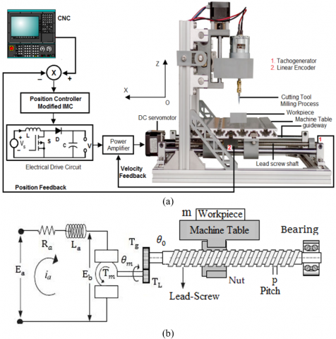
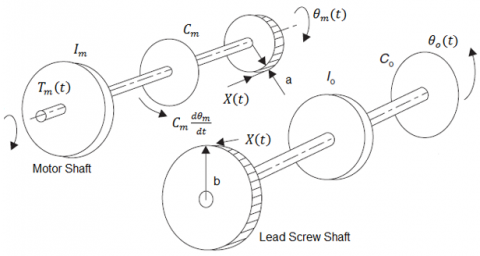
The physical configuration and Mechatronic diagram of the CNCMT system are shown in Figure 1 (a) and (b) respectively [22]. The block diagram of CNCMT systems is shown in Figure 2, and the parameters of blocks shown in the same are derived in Appendix-A.
The input to the CNCMT is electric power to the power amplifier which gives the suitable voltage applied to the servo motor and the output variables are position, velocity, and acceleration of the machine table. The position and velocity of the machine table are considered as output variables of the CNCMT system in this paper. In this work two feedback loops are employed which has the advantage to reduce the OS and is used where it is undesirable like in cutting and welding operations. The friction due to lead screw shaft is very less as compared to friction due to drilling, boring and milling operations in the CNCMT system. Therefore, assuming the lead screw shaft is friction-free. The detailed mathematical modeling of the CNCMT system is presented in appendix-A. The nominal values and the range of parametric uncertainty of the CNCMT system used in simulation and stability analysis are given in Table 1. The equivalent inertia (Im) i.e. combined inertia of motor shaft and lead screw shaft, weight/mass of workpiece (m), gains of the power amplifier (K1), and servomotor (K2) are considered as uncertain parameters as shown in Table 1. Because under running conditions inertia of the motor are varying, and the parameters related to gains of power amplifier and servomotor are changing under varying environmental conditions. Therefore, these parametric uncertainties are considered in this study. From Figure 2, the transfer function of CNCMT system G(s) is represented by (1).
$G(s)=\frac{X_{0}(s)}{U(s)}=\frac{K_{1} K_{2} n p}{\left(p^{2} m+n^{2} I_{m}\right) s^{2}+K_{1} K_{2} n H_{2} s}=\frac{K_{1} K_{2} n p /\left(p^{2} m+n^{2} I_{m}\right)}{s^{2}+\frac{K_{1} K_{2} n H_{2}}{\left(p^{2} m+n^{2} I_{m}\right)} s}$ (1)
where, p is the pitch of lead screw, n is gear ratio, H1 is the gain of encoder and H2 is the gain of tach generator. X0(s) is the actual position of the machine table on the lead screw shaft which is coupled with the shaft of DC servo motor through the gearbox, and ‘s’ refers to Laplace function. In real or practical applications any system may be approximated as first or second-order plus delay time model, hence the open-loop transfer function of the CNCMT system is achieved after putting the values in (1) from Table 1, which is as follows:
$G(s)=\frac{X_{0}(s)}{U(s)}=\frac{4.85}{s(s+9.7)} * e^{-T_{d} s}$ (2)
where, Td is the delay time Td=0.1 is considered for simulation while in robustness analysis it is neglected for easy calculation.
It is clear from (2) that there is one pole at origin i.e. integrator type, hence open-loop system is marginally stable. The location of poles depends upon machine parameters which have uncertainty; hence it is required to design a robust controller that improves the system performance. In this research, the robust PI, IMC, and H∞ controllers are taken into consideration for the desired position of the machine table on the lead screw shaft.
Table 1. Nominal values and uncertainty in CNCMT parameters
|
Description (SI unit) |
Symbol |
Uncertainty (%) |
|
Power Amp. gain (V/V) |
K1 |
2 ±50% |
|
Servomotor gain (Nm/V) |
K2 |
4 ±25% |
|
Mass of workpiece (kg) |
m |
50±40% |
|
Equivalent inertia (kg-m2) |
Im |
0.01±20% |
|
Pitch of lead screw (mm) |
p |
5 |
|
Gear ratio |
n |
2:1 |
|
Gain of encoder |
H1 |
1 |
|
Gain of tachogenrator |
H2 |
0.1 |
Figure 1. (a) Physical configuration of CNCMT systems [22]; (b) Mechatronic diagram of CNCMT systems
Figure 2. Block diagram of CNCMT systems
3.1 Kharitonov’s theorem
The polynomial:
$P(s)=\sum_{i=0}^{n} a_{i} s^{n-i}=a_{0} s^{n}+a_{1} s^{n-1}+a_{2} s^{n-2}+\cdots+a_{n-1} s+a_{n}$ (3)
where, $\alpha_{i} \leq a_{i} \leq \beta_{i}, 0 \leq i \leq n$, and αiand βi are lower and upper limit values of polynomial respectively.
Kharitonov’s theorem says that the P(s) is stable if four polynomials as given by (4) are stable.
$p_{1}(s)=\alpha_{0} s^{n}+\alpha_{1} s^{n-1}+\beta_{2} s^{n-2}+\beta_{3} s^{n-3}+\cdots$
$p_{2}(s)=\alpha_{0} s^{n}+\beta_{1} s^{n-1}+\beta_{2} s^{n-2}+\alpha_{3} s^{n-3}+\cdots$
$p_{3}(s)=\beta_{0} s^{n}+\alpha_{1} s^{n-1}+\alpha_{2} s^{n-2}+\beta_{3} s^{n-3}+\cdots$
$p_{4}(s)=\beta_{0} s^{n}+\beta_{1} s^{n-1}+\alpha_{2} s^{n-2}+\alpha_{3} s^{n-3}+\cdots$ (4)
The necessary and sufficient condition for robust stability of the third-order system and formula for calculation of SM is given by Hote et al. [14] which is as follows:
$\alpha_{1} \alpha_{2}>\beta_{0} \beta_{3}$ and $S M=\alpha_{1} \alpha_{2}-\beta_{0} \beta_{3}$ (5)
Hence, if the SM is high i.e. more positive, then the system will be more stable, if the SM is zero, then the system is marginally stable, otherwise, the system will be unstable.
3.2 Design of controller using the worst GM and PM
The closed-loop characteristic equation (CLCE) with controller C(s) is written as
$1+G(s) C(s)=0$ (6)
In order to determine the GM, a virtual gain kv is introduced in series with G(s). Therefore, the CLCE in the form of a polynomial can be written as;
$P(s)=a_{0} s^{3}+a_{1} s^{2}+a_{2} s+a_{3} k_{v}$ (7)
The GM of the system is calculated simply from the s1 row of the Routh array and the phase crossover frequency ѡcp is determined using an auxiliary equation which is derived from the s2 row. Considering p3(s) because it gives the worst value of GM and PM [9, 10] the equation for p3(s) of (4) using (7) is as follows:
$p_{3}(s)=\beta_{0} s^{3}+\alpha_{1} s^{2}+\alpha_{2} s+\beta_{3} k_{v}$ (8)
Formulate the Routh table and taking higher-order coefficient is equal to 1.
|
s3 |
1 |
$\alpha_{1}$ |
|
s2 |
α2 |
$\beta_{3} k_{v}$ |
|
s1 |
$\left(\alpha_{1} \alpha_{2}-\beta_{3} k_{v}\right) / \alpha_{2}$ |
0 |
|
s0 |
$\beta_{3} k_{v 1}$ |
0 |
From s1 row of above Routh table,
$\left(\alpha_{1} \alpha_{2}-\beta_{3} k_{v}\right) / \alpha_{2}=0$ (9)
$k_{v}=\frac{\alpha_{1} \alpha_{2}}{\beta_{3}}=\frac{\text { coefficient of } s^{2} \times \text { coefficient of } s^{1}}{\text { coefficient of } s^{0}}$ (10)
$\mathrm{GM}$ in $\mathrm{dB}=20 \log \frac{\alpha_{1} \alpha_{2}}{\beta_{3}}$ (11)
The auxiliary equation, from s2 row of Routh table, is written as:
$\alpha_{2} S^{2}+\beta_{3} k_{v}=0$ (12)
Put s=jw and $k_{v}=\frac{\alpha_{1} \alpha_{2}}{\beta_{3}}$ in (12), it gives wcp
$\omega=\omega_{c p}=\sqrt{\alpha_{2}}=\sqrt{\text { coefficient of } s^{1}}$ (13)
In order to determine the PM, gain crossover frequency wcg is determined first which is calculated using the empirical formula as given by [10]:
$\omega_{c g}=\omega_{c p}\left(\frac{1}{k_{v}}\right)^{0.5}$ (14)
From (10), (13), and (14); $\omega_{c g}=\sqrt{\beta_{3} / \alpha_{1}}$ and PM is as follows:
$P M=180^{0}-90^{0}-\tan ^{-1}\left(\sqrt{\alpha_{1}^{3} * \beta_{3}} /\left(\alpha_{1} \alpha_{2}-\beta_{3}\right)\right)$ (15)
In recent research, the typical range of GM and PM is 5-10dB and 50°-70° respectively. To design a robust PI controller the 10 dB of GM and 60° of PM is considered in this paper. From (1) and (6) the CLCE with PI controller can be written as:
$1+\left(\frac{\frac{K_{1} K_{2} n p}{\left(p^{2} m+n^{2} I_{m}\right)}}{s^{2}+\frac{K_{1} K_{2} n H_{2}}{\left(p^{2} m+n^{2} I_{m}\right)} s}\right)\left(K_{P}+\frac{K_{I}}{s}\right)=0$ (16)
where, KP and KI are parameters of the PI controller. Formulate a polynomial p(s) using p3(s) of (4), (16) and values from Table 1, yields (17).
$p(s)=s^{3}+7.5 s^{2}+3 K_{P} s+6 K_{I}$ (17)
The lower and upper limit values of (17) are as follows: α1=7.5, α2=3 and β0=1, β3=6 respectively.
From (11) and (17),
$G M=20 \log \frac{7.5 * 3 * K_{P}}{6 K_{I}}=10 \Rightarrow K_{P}=0.84 * K_{I}$ (18)
From (15) and (17),
$P M=180^{\circ}-90^{\circ}-\tan ^{-1}\left(\frac{\sqrt{7.5^{3} * 6 * K_{I}}}{7.5 * 3 * K_{P}-6 K_{I}}\right)=60^{\circ}\Rightarrow\left(22.5 K_{P}-6 K_{I}\right)^{2}=7593.75 * K_{I}$ (19)
After solving (18) and (19); we obtain Kp=38.33 and K1=45.65.
3.3 IMC design theory
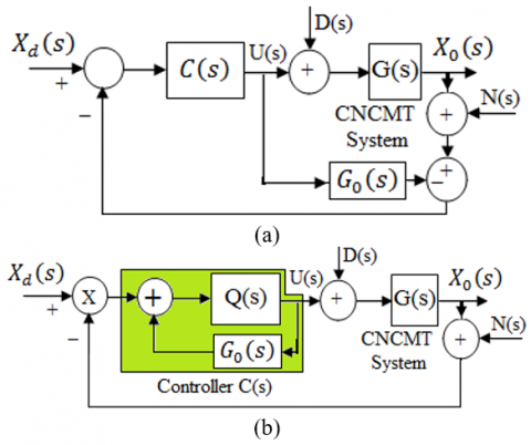
IMC has many features such as noise and disturbance rejection capability, tracking of reference trajectory, and insensitive to parameter variations i.e. it makes a robust system [22]. In IMC, a single tunable parameter μ exists as given in (22). The procedure to obtain the suitable value of μ is discussed in appendix-B. The controller parameter μ represents a trade-off between tracking performance and robustness of the system and this is a unique feature of IMC. The generalized architecture of IMC is presented in Figure 3(a) and the proposed simplified IMC block diagram is shown in Figure 3(b), which gives similar performance as given by the IMC as shown in Figure 3(a). It consists of controller C(s), original system (G(s)), and internal model G0(s). D(s) and N(s) are disturbance and noise in the system respectively.
Figure 3. (a) Generalized architecture (b) Proposed block diagram of IMC
From Figure 3(b); considering D(s) and N(s) are equal to zero.
$X_{0}(s)=\frac{G(s) C(s) X_{d}(s)}{1+C(s) G(s)}$ (20)
$C(s)=\frac{Q(s)}{1-G_{0}(s) Q(s)}$ (21)
The condition for perfect reference point tracking and effect of parameter variations are obtained, if G0(s)=G(s) and Q(s)=1/G(s) [18, 22]. If G(s) is proper, then it's inverse i.e. 1/G(s) becomes improper. Hence to make a proper system a low pass filter is incorporated as a part of Q(s). Hence it is defined as:
$Q(s)=\frac{1}{(\mu s+1)^{\lambda}} G(s)^{-1}$ (22)
where, λ is the value which makes Q(s) proper. The low pass filter parameter μ influences the speed of response and robustness of the system. Here taking λ=2 and μ=1 for the design of IMC. The selection procedure of the suitable value of μ for different operations of the CNCMT system is discussed in appendix-B. Therefore, the transfer function of IMC is as follows:
$C(s)=\frac{0.21 s+2}{s+2}$ (23)
3.4 H∞ control technique
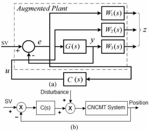
The standard configuration of H∞ control with weighting functions W1, W2, and W3, and the proposed robust control block for uncertain CNCMT system is shown in Figure 4 (a) and (b) respectively. The motive of controller C(s) is to obtain both tracking and robustness performances under a specified range of system parameters.
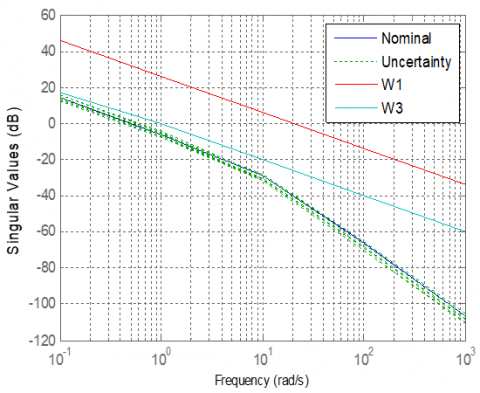
In Figure 4(a), G(s) is the system with nominal values; z, y, SV, and u are the controlled output, the measured output, the set value, and the control input respectively, whereas of W1(s), W2(s) and W3(s) are weights to the tracking error, controller transfer function, and system performance respectively. Figure 5 depicts the variation of singular values of the nominal system, plant uncertainty, and weighting function W1 and W3 with low to high frequency.
Figure 4. (a) Standard configuration of H∞ control with W1, W2, and W3 weighting functions; (b) Proposed robust control block diagram for uncertain CNCMT system
Figure 5. Plot of singular values of the nominal system, plant uncertainty, and W1 and W3
The C(s) is designed such that the H∞ norm of the sensitivity matrix ||S(jω)||∞ and the mixed-sensitivity matrix, ||M(jω)||∞ are minimized, where M(jω) is given by the following equation [13, 25].
$M(j \omega)=\left[\begin{array}{c}W_{1}(j \omega) S(j \omega) \\ W_{2}(j \omega) C(j \omega) S(j \omega) \\ W_{3}(j \omega) T(j \omega)\end{array}\right]$ (24)
The weighting matrices for tracking and robustness performance of H∞ control is represented as follows [25]:
$\sigma_{\max }(S(j \omega)) \leq \sigma_{\max }\left(W_{1}^{-1}(j \omega)\right)$
$\sigma_{\max }(C(j \omega) S(j \omega)) \leq \sigma_{\max }\left(W_{2}^{-1}(j \omega)\right)$
$\sigma_{\max }(T(j \omega)) \leq \sigma_{\max }\left(W_{3}^{-1}(j \omega)\right)$ (25)
where, σmax is the maximum singular value. The H∞ control algorithm used in this work is as follows:
$\|\vartheta M(j \omega)\|_{\infty} \leq 1$ (26)
where, ϑ is a scaling factor. Using a robust control toolbox of MATLAB command ‘hinfopt’ which iterates ϑ until a stabilizing solution which satisfies (26) is obtained. The selection of W1(s), W2(s), and W3(s) are determined with the help of Yang et al. [26]. The weighting transfer functions used in the simulation are given as below:
$W_{1}(s)=\frac{20}{s+0.01}, W_{2}(s)=1$ and $W_{3}(s)=\frac{1}{s+0.1}$ (27)
Iteration number 14 gives an answer under the tolerance of 0.0100, which has ϑ=1.3794*10-2. The order of the resulting controller is fourth, which is the same as the order of the augmented plant. The stabilizing C(s) is obtained as follows:
$C(s)=\frac{20.12 s^{3}+197.2 s^{2}+19.52 s+2.72 * 10^{-13}}{s^{4}+14.23 s^{3}+54.16 s^{2}+5.879 s+0.05339}$ (28)
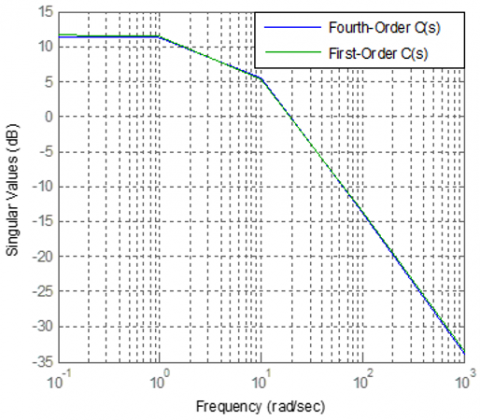
Using order reduction command ‘reduce' of MATLAB, the original controller given by (28) is reduced to the first order for easy calculation of robust stability. The reduced-order controller gives almost similar performance as the original higher-order controller. The original and reduced order controller gives almost the same singular value from low to high-frequency range as shown in Figure 6.
Figure 6. Plot of singular values of original forth and reduced first-order controller C(s)
The transfer function of reduced first order stabilized controller C(s) is as follows:
$C(s)=\frac{20.97}{s+5.5}$ (29)
3.5 Robustness analysis of uncertain CNCMT system in terms of SM
The robust stability analysis of uncertain CNCMT systems with robust PI, IMC, and H∞ controllers, and using the Kharitonov theorem is presented in this section. For the robust stability analysis and calculation of SM, it is required to calculate the α1, α2, β0 and β3 as represented in (5). The CLCE of CNCMT system with a robust PI controller is as follows:
$s^{3}+\frac{K_{1} K_{2} n H_{2}}{\left(p^{2} m+n^{2} I_{m}\right)} s^{2}+\frac{K_{1} K_{2} n p}{\left(p^{2} m+n^{2} I_{m}\right)} K_{P} s+\frac{K_{1} K_{2} n p}{\left(p^{2} m+n^{2} I_{m}\right)} K_{I}=0$ (30)
where, Kp=38.33, K1=45.65, and β0=1. The uncertainty of CNCMT system parameters as shown in Table 1 is used for calculation of α1, α2, and β3 as shown below:
$\alpha_{1}=\min \left\{\frac{K_{1} K_{2} n H_{2}}{\left(p^{2} m+n^{2} I_{m}\right)}\right\}=7.5$
$\alpha_{2}=\min \left\{\frac{K_{1} K_{2} n p}{\left(p^{2} m+n^{2} I_{m}\right)} K_{P}\right\}=115$ and
$\beta_{3}=\max \left\{\frac{K_{1} K_{2} n p}{\left(p^{2} m+n^{2} I_{m}\right)} K_{I}\right\}=273.9$ (31)
With these values satisfying the condition (5); gives 7.5*15>273.89, hence the system is found stable. From (5) SM is calculated as 588.6.
The CLCE with IMC is given by (32).
$s^{3}+\left\{2+\frac{K_{1} K_{2} n H_{2}}{\left(p^{2} m+n^{2} I_{m}\right)}\right\} s^{2}$
$+\left\{2 * \frac{K_{1} K_{2} n H_{2}}{\left(p^{2} m+n^{2} I_{m}\right)}+0.21\right.$
$\left.* \frac{K_{1} K_{2} n p}{\left(p^{2} m+n^{2} I_{m}\right)}\right\} s+2$
$* \frac{K_{1} K_{2} n p}{\left(p^{2} m+n^{2} I_{m}\right)}=0$ (32)
The values of α1, α2, and β3 are calculated and as given below:
$\alpha_{1}=\min \left\{2+\frac{K_{1} K_{2} n H_{2}}{\left(p^{2} m+n^{2} I_{m}\right)}\right\}=9.5$,
$\alpha_{2}=\min \left\{2 * \frac{K_{1} K_{2} n H_{2}}{\left(p^{2} m+n^{2} I_{m}\right)}+0.21 * \frac{K_{1} K_{2} n p}{\left(p^{2} m+n^{2} I_{m}\right)}\right\}=16.575$
and $\beta_{3}=\max \left\{2 * \frac{K_{1} K_{2} n p}{\left(p^{2} m+n^{2} I_{m}\right)}\right\}=12$ (33)
The stability condition as given by (5) is satisfied; therefore, the uncertain system is found as stable. The SM from (5) is calculated as 9.5*16.575-12=145.4.
The CLCE with H∞ controller is as follows:
$s^{3}+\left\{5.5+\frac{K_{1} K_{2} n H_{2}}{\left(p^{2} m+n^{2} I_{m}\right)}\right\} s^{2}+\left\{5.5 * \frac{K_{1} K_{2} n H_{2}}{\left(p^{2} m+n^{2} I_{m}\right)}\right\} s+20.97 * \frac{K_{1} K_{2} n p}{\left(p^{2} m+n^{2} I_{m}\right)}=0$ (34)
The values of α1, α2, and β3 are calculated and as given below:
$\alpha_{1}=\min \left\{5.5+\frac{K_{1} K_{2} n H_{2}}{\left(p^{2} m+n^{2} I_{m}\right)}\right\}=13$
$\alpha_{2}=\min \left\{5.5 * \frac{K_{1} K_{2} n H_{2}}{\left(p^{2} m+n^{2} I_{m}\right)}\right\}=41.25$ and
$\beta_{3}=\max \left\{20.97 * \frac{K_{1} K_{2} n p}{\left(p^{2} m+n^{2} I_{m}\right)}\right\}=125.82$ (35)
The stability condition is given by (5) is satisfied; hence the uncertain system is stable. The SM is calculated as follows: 13*41.25-125.82=410.4, which is slightly less than as obtained using a robust PI controller but it is much more than that obtained using IMC. With high SM controller can handle a wider range of parametric uncertainty in the CNCMT system.
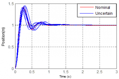
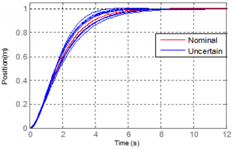
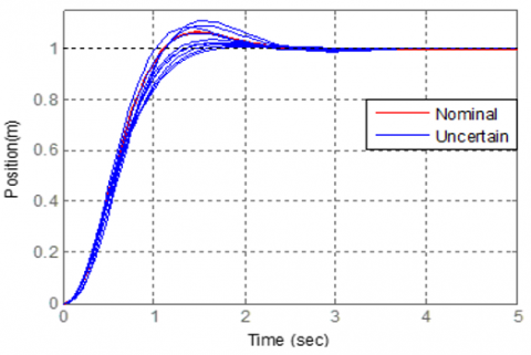
The results obtained using MATLAB simulations are presented in this section. The response of uncertain CNCMT systems with robust PI, IMC, and H∞ controllers are presented and compared. Figures 7 to 9, show the step response of the CNCMT system with robust PI, IMC, and H∞ controllers respectively.
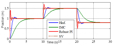
The response Figures 7 to 9 are plotted after considering 10 uncertain samples between the lower and upper limit via nominal values as given in Table 1. The performance index of nominal and uncertain CNCMT system with all designed controllers is given in Table 2. From Figures 7-9 and Table 2, it is evident that the H∞ controller gives the narrowest OS, ST, and RT bands as compared to robust PI and IMC, meaning that the narrower bands give a similar performance under parameter variations, i.e., the robustness of the uncertain CNCMT system towards the parametric uncertainty is achieved with the H∞ controller. Hence H∞ controller gives better performances as compared to robust PI and IMC for uncertain CNCMT systems.
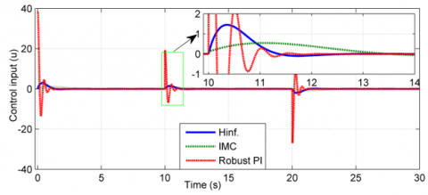
Figure 10 shows the combined response of nominal system parameters with all designed controllers for comparative performance analysis. Figure 11 shows the response of the controller output of robust PI, IMC, and H∞ control techniques for the CNCMT system. From Figure 11, it is evident that the IMC gives the least and sluggish control effort, H∞ control gives moderate and fast control effort whereas robust PI controller gives high output that implies it requires much control effort for the regulation of the desired position of the CNCMT system.
Figure 7. Step response of uncertain CNCMT system with robust PI controller
Figure 8. Step response of uncertain CNCMT system with IMC controller
Figure 9. Step response of uncertain CNC system with H∞ controller
Table 2. Performance index of nominal and uncertain system
|
Performance Parameters |
|||||
|
Controller |
OS (%) |
ST (s) |
RT (s) |
SM |
|
|
Robust PI |
Nominal |
41.2 |
0.88 |
0.14 |
588.6 |
|
Uncertain |
32.8-45.3 |
0.77-1.33 |
0.123-0.27 |
||
|
IMC |
Nominal |
0.57 ≃ 0 |
5.84 |
3.36 |
145.46 |
|
Uncertain |
0.12-1.27 |
4.1-7.08 |
2.56-3.98 |
||
|
H∞ |
Nominal |
6.3 |
2.09 |
1.12 |
410.43 |
|
Uncertain |
0.598-10.9 |
1.34-2.32 |
1.02-1.74 |
||
Figure 10. The combined response of CNCMT system with all designed controllers
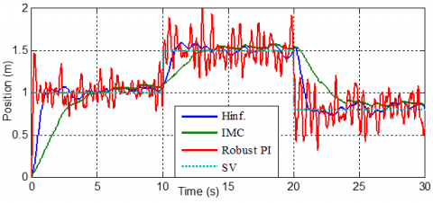
Figure 12 shows the input disturbance and non-deterministic noise in the system. The variation in input voltage is considered as input disturbance and noise due to the sensor i.e. sensory noise is usually generated during the measurement is considered in this paper. These disturbances and noise are used for showing the response Figure 13, which is the combined response of the CNCMT system in the influence of disturbance and noise with all designed controllers. The proposed H∞ controller gives better input disturbance and sensor noise rejection capability as clearly seen in Figure 13.
Figure 11. Controlled input response of all designed controllers for CNCMT system
Figure 12. Input disturbances and noise signal after the sensor unit
Figure 13. Response with input disturbance and sensor noise
From Figure 10, it is evident that the robust PI controller gives the least ST and RT and very high OS and better SM as compared to IMC and H∞ controllers. High OS is harmful, which is unwanted energy and cannot be tolerated for cutting operations in CNC machines. IMC gives nearly zero OS, but it gives the least SM and more RT and ST as compared to robust PI and H∞ controllers, which indicates sluggish CNC machine operations. H∞ controller gives all the performance parameters such as OS, ST, RT, and SM under design consideration and suitable for all CNC machine tool operations such as drilling, cutting, milling, boring, finishing, aligning etc. According to the proper balance of performance parameters, H∞ controller is best amongst the other designed controllers.
In this paper the robust PI, IMC, and H∞ controllers are designed successfully for uncertain CNCMT system that is subjected to input disturbance and sensor noise. Comparative performance analysis of the controllers is performed and shows that H∞ controller gives a better and desirable performance index and reasonable SM among all other reported controllers. H∞ controller and IMC have eliminated measurement noise and disturbance completely as compared to the robust PI controller. Hence H∞ controller is considered best out of other designed controllers in this paper. This robust control technique may also be applied to aerospace and other electromechanical systems.
|
Acronyms |
|
|
CLCE |
closed-loop characteristic equation |
|
CNC |
computerized numeric controlled |
|
CNCMT |
computerized numeric controlled machine tool |
|
GM |
gain margin |
|
IMC |
internal model control |
|
OS |
overshoot |
|
PI |
proportional-integral |
|
PM |
phase margin |
|
RT |
rise time |
|
SM |
stability margin |
|
ST |
settling time |
|
Symbols |
|
|
C(s) |
Controller |
|
H1 |
the gain of shaft encoder |
|
H2 |
gain of tachogenrator |
|
Im |
equivalent inertia (kg-m2) |
|
K1 |
power amplifier gain (V/V) |
|
K2 |
servomotor gain (Nm/V) |
|
KP |
proportional gain of PI controller |
|
KI |
integral gain of PI controller |
|
m |
mass of work piece (kg) |
|
n |
gear ratio |
|
p |
pitch of lead screw (m) |
|
$T_{d}$ |
delay time (s) |
|
W1, W2, W3 |
weighting functions |
|
$\lambda, \mu$ |
filter parameters of IMC |
This section presents the modeling of the CNCMT system and derivation of the transfer function of the same as represented by (1). Consider Figures 1 and 2 for the complete modeling of the CNCMT system [4].
1. Power Amplifier: The output of the power amplifier is a controlled input E(s) to the DC servomotor as follows:
$E(s)=K_{1}(U(s)-B(s))$ (36)
where, K1 is the gain of the power amplifier.
2. DC servo motor: The applied voltage e(t) is described as follows:
$e(t)=L_{f} \frac{d i_{f}}{d t}+R_{f} i_{f}$ (37)
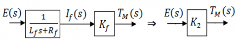
where, Lf and Rf are the motor parameters, and if is the field current. The motor torque Tm $\propto i_{a} i_{f}$, since $i_{a}$ is constant for field controlled DC motor, therefore Tm=Kf if, where Kf is the constant. Assuming field time constant Lf/Rf is small as compared to the mechanical time constant of the motor. Therefore, Tm is as follows:
$T_{M}(s)=K_{2} E(s)$ (38)
The equivalent block diagram of field controlled DC servo motor is shown in Figure 14.
Figure 14. Equivalent field controlled DC servo motor
3. Gearbox, Lead Screw, and Machine Table: The free body diagram of the gearbox with motor and lead screw shafts are shown in Figure 15.
Figure 15. Free body diagram of the gearbox with motor and lead screw shafts
For the motor shaft:
$\sum M=I_{m} \frac{d^{2} \theta_{m}}{d t^{2}}$ (39)
$T_{m}(t)-C_{m} \frac{d \theta_{m}}{d t}-a X(t)=I_{m} \frac{d^{2} \theta_{m}}{d t^{2}}$ (40)
where, X(t) is gear tooth reaction force, θm is the angular position of the motor, a is the radius of gear connected to the motor and Im is the equivalent inertia of the motor. Rearranging (40),
$X(t)=\frac{1}{a}\left(T_{m}(t)-C_{m} \frac{d \theta_{m}}{d t}-I_{m} \frac{d^{2} \theta_{m}}{d t^{2}}\right)$ (41)
Taking Laplace transform of (41) with Cm=0.
$X(s)=\frac{1}{a}\left(T_{m}(s)-I_{m} s^{2} \theta_{m}(s)\right)$ (42)
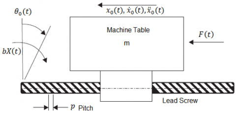
The Free body diagram of the machine table and lead screw shaft is shown in Figure16.
For lead screw shaft assuming: work in = workout.
$b X(t) \theta_{0}(t)=F(t) x_{0}(t)$ (43)
where, b is the radius of gear connected to the lead screw shaft, θ0 is the angular position of lead screw, F(t) is the force acting on the machine table and x0 is the linear position of the machine table.
Figure 16. Free body diagram of the machine table and lead screw shaft
The pitch p of the lead screw is defined as:
$p=\frac{x_{0}(t)}{\theta_{0}(t)}$ (44)
From (43) and (44),
$F(t)=\frac{b X(T)}{p}$ (45)
The equation of motion for the machine table is written as follows:
$F(t)=m \ddot{x}_{0}$ (46)
Equating (45) and (46) and taking Laplace transform.
$X(s)=\frac{1}{b}\left(p m s^{2} X_{0}(s)\right)$ (47)
Equating (42) and (47) gives (48).
$p m s^{2} X_{0}(s)=\frac{b}{a}\left(T_{m}(s)-I_{m} s^{2} \theta_{m}(s)\right)$ (48)
where, $\frac{b}{a}=n$ i.e. gear ratio and
$\theta_{m}(s)=n \theta_{0}(s)$ (49)
Hence,
$s^{2} \theta_{m}(s)=n s^{2} \theta_{0}(s)$ (50)
From (44),
$G_{0}(s)=\frac{X_{0}(s)}{p}$ (51)
From (48) to (51),
$p m s^{2} X_{0}(s)=n T_{m}(s)-n I_{m} \frac{n}{p} s^{2} X_{0}(s)$ (52)
Hence the open-loop transfer function of the gearbox, lead screw, and machine table is obtained after rearranging (52), which is as follows:
$\frac{s X_{0}(s)}{T_{m}(s)}=\frac{n}{\left(p m+\frac{n^{2} I_{m}}{p}\right) s}$ (53)
4. Tachogenerator: The feedback signal B(s) is given as:
$B(s)=H_{2} s \theta_{0}(s)$ or $B(s)=H_{2} s X_{0}(s) / p$ (54)
where, H2 is the gain of tachogenerator.
5. Position transducer: Feedback signal Xm(s) is given as follows:
$X_{d}(s)=H_{1} X_{0}(s)$ (55)
where, H1 is the gain of shaft encoder. The overall system is represented in Figure 2 is a block diagram of the CNCMT system. The complete open-loop transfer function of the CNCMT system is given by (1).
This appendix presents the investigative approach for the selection of adjustable parameter μ of IMC. Let us consider a generlized second order system as given below:
$G(s)=\frac{k}{s^{2}+d_{1} s+d_{0}}$ (56)
and from (21);
$C(s)=\frac{Q(s)}{1-G_{0}(s) * Q(s)}$ (57)
where, $Q(s)=\frac{1}{(\mu s+1)^{n}} G(s)^{-1}$ and $G_{0}(s)=G(s)$
For $n=2, C(s)=\frac{s^{2}+d_{1} s+d_{0}}{k\left(\mu^{2} s^{2}+2 \mu s\right)}$ (58)
The CLCE is 1+G(s)C(s)=0, that becomes (59) after putting the values of G(s) and C(s) from (56) and (58) respectively.
$s^{2}+\frac{2}{\mu} s+\frac{1}{\mu^{2}}=0$ (59)
Comparing (59) with standard second order characteristic equation i.e. $s^{2}+2 \xi \omega_{n} s+\omega_{n}^{2}=0$, gives ξ=1 and $\omega_{n}=\frac{1}{\mu}$. A performance Table 3 is used for the selection of suitable value of μ.
Table 3. Performance parameters for different values of μ
|
μ |
$\xi$ |
ωn |
$\mathbf{D P}=-\xi \omega_{n} \pm j \omega_{n} \sqrt{\left(1-\xi^{2}\right)}$ |
ST =4/ξωn |
OS |
|
0.1 |
1 |
10 |
-10 |
0.4 |
0 |
|
1.0 |
1 |
1 |
-1 |
4 |
0 |
|
10 |
1 |
0.1 |
-0.1 |
40 |
0 |
The selection of the desired value of μ requires a proper balance of bandwidth, ST, RT, sensitivity, and control efforts, etc. Hence according to the proper balance of performance parameters as derived in Table 3, μ=1 is the best out of the three given values as 0.1, 1, and 10.
[1] Huang, W.S., Liu, C.W., Hsu, P.L., Yeh, S.S. (2010). Precision control and compensation of servomotors and machine tools via the disturbance observer. IEEE Transactions on Industrial Electronics, 57(1): 420-429. https://doi.org/10.1109/TIE.2009.2034178
[2] Jee, S., Koren, Y. (2004). Adaptive fuzzy logic controller for feed drives of a CNC machine tool. Mechatronics, 14(3): 299-326. https://doi.org/10.1016/S0957-4158(03)00031-X
[3] Xiao, N., Liu, Y., Zhang, X., Liu, Y. (2020). Swing angle error compensation of a computer numerical control machining center for special-shaped rocks. Journal Européen des Systèmes Automatisés, 53(3): 369-375. https://doi.org/10.18280/jesa.530307
[4] Burns, R.S. (2001). Advanced Control Engineering: Closed-Loop Control Systems. Burrerworth-Heinemann, First Edition, Jordan Hill, Oxford, 63-109.
[5] Li, Z.Z., Sato, R., Shirase, K., Ihara, Y., Milutinovic, D.S. (2019). Sensitivity analysis of relationship between error motions and machined shape errors in five-axis machining center - peripheral milling using square-end mill as test case. Precision Engineering, 60: 28-41. https://doi.org/10.1016/j.precisioneng.2019.07.006
[6] Hou, Y., Zhang, D., Mei, J., Zhang, Y., Luo, M. (2019). Geometric modelling of thin-walled blade based on compensation method of machining error and design intent. Journal of Manufacturing Processes, 44: 327-336. https://doi.org/10.1016/j.jmapro.2019.06.012
[7] An, S., Liu, W. (2004). Robust D-stability with mixed-type uncertainties. IEEE Transactions on Automatic Control, 49(10): 1878-1884. https://doi.org/10.1109/TAC.2004.835594
[8] Bhattacharyya, S.P., Datta, A., Keel, L.H. (2009). Linear Control Theory: Structure, Robustness and Optimization. CRC Press, Taylor and Francis Group, New York.
[9] Yadav, A.K., Gaur, P., Saxena, P. (2016). Robust stability analysis of PMSM with parametric uncertainty using Kharitonov theorem. Journal of Electrical Systems, 12(2): 258-277.
[10] Hote, Y.V., Gupta, J.R.P., Choudhury, D.R. (2010). Kharitonov’s theorem and Routh criterion for stability margin of interval systems. International Journal of Control, Automation, and Systems, 8(3): 647-654. https://doi.org/10.1007/s12555-010-0318-1
[11] Kharitonov, V.L. (1978). Asymptotic stability of an equilibrium position of family of linear differential equation. Differensialnye Uravneniya, 14: 2086-2088.
[12] Meressi, T., Chen, D., Paden, B. (1993). Application of Kharitonov’s theorem to Mechanical Systems. IEEE Trans. on Automatic Control, 38(3): 488-491. https://doi.org/10.1109/9.210153
[13] Yadav, A.K., Gaur, P. (2014). Robust adaptive speed control of uncertain hybrid electric vehicle using electronic throttle control with varying road grade. Nonlinear Dynamics, 76(1): 305-321. https://doi.org/10.1007/s11071-013-1128-9
[14] Hote, Y.V., Choudhury, D.R., Gupta J.R.P. (2009). Robust stability analysis of a PWM push-pull DC-DC converter. IEEE Transaction on Power Electronics, 24(10): 2353-2356. https://doi.org/10.1109/TPEL.2009.2014132
[15] Sharma, J., Hote, Y.V., Prasad, R. (2019). PID controller design for interval load frequency control system with communication time delay. Control Engineering Practice, 89: 154-168. https://doi.org/10.1016/j.conengprac.2019.05.016
[16] Garcia, C.E., Morari, M. (1982). Internal model control-1: A unifying review and some new results. Ind. Eng. Chem. Process Design Development, 21(2): 308-323. https://doi.org/10.1021/i200017a016
[17] Yadav, A.K., Gaur, P. (2015). Intelligent modified internal model control for speed control of nonlinear uncertain heavy duty vehicles. ISA Transactions, 56(3): 288-298. https://doi.org/10.1016/j.isatra.2014.12.001
[18] Liu, T., Gao, F. (2010). New insight into internal model control filter design for load disturbance rejection. IET Control Theory Application, 4(3): 448-460. https://doi.org/10.1049/iet-cta.2008.0472
[19] Yadav, A.K., Gaur, P. (2017). Speed control of an uncertain heavy duty vehicle using improved IMC technique. The Arabian Journal for Science and Engineering, 42(7): 2981–2991. https://doi.org/10.1007/s13369-017-2481-7
[20] Yadav, A.K., Gaur, P. (2016). Neuro-fuzzy based improved IMC for speed control of nonlinear heavy duty vehicles. Defence Science Journal, 66(6): 665-672. https://doi.org/10.14429/dsj.66.9489
[21] Saxena, S., Hote, Y.V. (2013). Load frequency control in power systems via internal model control scheme and model-order reduction. IEEE Transactions on Power Systems, 28(3): 2749-2757. https://doi.org/10.1109/TPWRS.2013.2245349
[22] Yadav, A.K., Gaur, P. (2020). Modified IMC technique for nonlinear uncertain milling CNC machine tool system. The Arabian Journal for Science and Engineering, 45(3): 2065-2080. https://doi.org/10.1007/s13369-019-03984-7
[23] Glover, K., Doyle, J.C. (1988). State space formulae for all stabilizing controllers that satisfy an H∞ norm bound and relations to risk sensitivity. Systems and Control Letters, 11(3): 167-172. https://doi.org/10.1016/0167-6911(88)90055-2
[24] Ortega, M.G., Rubio, F.R. (2004). Systematic design of weighting matrices for the H∞ mixed sensitivity problem. Journal of Process Control, 14(1): 89-98. https://doi.org/10.1016/S0959-1524(03)00035-0
[25] Tewari, A. (2002). Modern Control Design with MATLAB and SIMULINK. John Wiley & Sons., England.
[26] Yang, S., Lei, Q., Peng, F.Z., Qian, Z. (2011). A robust control scheme for grid-connected voltage-source inverters. IEEE Transactions on Industrial Electronics, 58(1): 202-212. https://doi.org/10.1109/TIE.2010.2045998
[27] Dehghania, A., Lanzona, A., Andersona, B.D.O. (2006). H∞ design to generalize internal model control. Automatica, 42(11): 1959-1968. https://doi.org/10.1016/j.automatica.2006.06.007
[28] Chen, D., Zhang, S., Pan, R., Fan, J. (2018). An identifying method with considering coupling relationship of geometric errors parameters of machine tools. Journal of Manufacturing Processes, 36: 535-549. https://doi.org/10.1016/j.jmapro.2018.10.019
[29] Kim, D., Jeon, D. (2011). Fuzzy-logic control of cutting forces in CNC milling processes using motor currents as indirect force sensors. Precision Engineering, 35(1): 143-52. https://doi.org/10.1016/j.precisioneng.2010.09.001