Kamel Hamitouche* | Samira Chekkal | Hocine Amimeur | Djamal Aouzellag
© 2020 IIETA. This article is published by IIETA and is licensed under the CC BY 4.0 license (http://creativecommons.org/licenses/by/4.0/).
OPEN ACCESS
In this paper modelling and analysis of stand-alone dual stator induction generator (DSIG) with non-identical parameters under a new method has been done. The induction machine has two sets of stator three-phase windings spatially shifted by 30 electrical degrees. One supplied power to the DC load via a rectifier bridge and AC capacitors, and the other was connected to the battery banks by an inverter to store energy and restore it to regulate the power of the first stator in weak wind. We develop the steady state model and show the performances of different configurations by the simulation results.
stand-alone wind energy conversion system, DSIG, non-identical stators, field-oriented control, MPPT, storage system
Renewable power generation is a suitable technology used to deliver energy locally to customers specially in remote regions [1]. Recently, wind generation systems are attracting great attentions as clean and safe renewable power sources. Wind generation can be operated by constant speed and variable-speed operations using power electronic converters [2]. The increase of wind power capacity and the reduction of maintenance costs have also made wind power systems more competitive in the energy market [3].
The wind conversion system is composed of minimum elements able to optimize the transfer of the wind energy. Ideally, only one turbine, one transmission shaft, one rotating electrical generator and unidirectional or bidirectional electronic converters are required [4, 5].
A renewed economic and technical interest in energy storage has been observed in recent years because of the increased number of unstable RES. A wide range of energy storage technologies is available today, which provide a large spectrum of performance and capacity for different application purposes [6]. Stand-alone wind energy systems often include batteries, because the available wind does not always produce the required quantities of power [7]. If wind power exceeds the load demand, the surplus can be stored in the batteries.
Induction generators have been employed to operate as wind turbine generators and small hydroelectric generators coupled to the grid or in isolated power systems [8-10], due to the practical advantages related to low maintenance cost, better transient performance, ability to operate without dc power supply for field excitation, good overload protection ability, and brushless construction [11-13].
In the last century, the research in the multiphase machine drives has grown significantly. Electric vehicles and railway traction, all-electric ships, more-electric aircraft, and wind power generation systems are areas where this research activity has taken place [14-17].
In the last decade, a new generation of self-excitation induction machine strongly emerged in AC applications. It constitutes of multi-stators topology. A dual stator induction generator (DSIG) belongs to this category and it brings a lot of advantages compared to the traditional three-phase induction generator such as the minimization of rotor losses and torque ripples, the reduction of harmonic, reducing current without increasing voltage in each phase and the power segmentation [18-20].
In the previous DSIG studies [12, 19-21], the machines were identical windings parameters and provide power in the same time; the DSIG presented in this study has different parameters and independent modes of operations.
The conventional configuration using only induction generator in wind power applications, consists to connect the battery bank directly to the DC bus voltage by bidirectional buck-boost converter, in this configuration, the battery bank stores the excess energy when the charge demand is low [22, 23].
To overcome this problem, in this paper, the battery bank is connected to a control winding through a dc/ac converter, thus the battery bank is charged at the same time as the load demand is supplied with its nominal value as long as the wind allows, furthermore the proposed configuration allows the main converter to transfer an almost constant power.
The DSIG presented in this paper has two sets of stator windings wound for the same number of pole pairs, their functions are different and separated, and they have no physical connection but have an electromagnetic link, one of which is called as power winding supplied 75% of the power of the DSIG to DC load via a bridge rectifier and self-excited capacitors, while the other is termed as control winding which provides 25% of the power to charge the battery bank by an inverter and restitute this energy to provide the power winding in case of weak wind as shown in Figure 1.
Moreover, like the traditional IG, the rotor of the DSIG is a cage type. It is simple, robust, and innate brushless, which can guarantee good safety and reliability of the DSIG.
Figure 1. Aerogenerator based on the DSIG
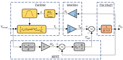
Figure 2. Block diagram of the wind turbine control loops
The power of the wind transferred to the rotor is calculated as follows [24]:
$P_{t}=\frac{1}{2} C_{p}(\lambda, \beta) \rho S V_{w i n d}^{3}$ (1)
where, $\rho$= 1.225 kg.m-3 is the mass density of the air at T~ 15℃ and $C_{p}(\lambda, \beta)$ is the turbine power coefficient that is a function of speed ratio λ and blade pitch angle ꞵ according [25]:
$C_{p}(\lambda, \beta)=C_{1} \cdot\left(\frac{C_{2}}{\lambda_{i}}-C_{3} \beta-C_{4}\right) \cdot \exp ^{-\left(\frac{C_{5}}{\lambda_{i}}\right)}+C_{6} \lambda_{i}$ (2)
where,
$\frac{1}{\lambda_{i}}=\frac{1}{\lambda+0.08 \beta}-\frac{0.035}{\beta^{3}+1}$ (3)
The parameters C1, C2, C3, C4, C5, C6, depend on the aerodynamic characteristics of the turbine. For a modern turbine these parameters are obtained empirically where: C1 = 0.5176, C2 = 116, C3 = 0.4, C4 = 5, C5 = 21, C6 = 0.0068, these values are given for a three-bladed wind turbine, with similar aerodynamic characteristics to the wind turbine model used in this system. The value of (ꞵ=0°) is to obtain the optimal tip speed ratio (λ) [26].
The speed ratio is given by:
$\lambda=\frac{R \Omega_{t}}{V_{\text {wind}}}$ (4)
And the Vwind is the wind speed assumed to be constant over the entire of the surface swept by rotor blade S.
The torque produced by the wind turbine is calculated by
$T_{t}=\frac{P_{t}}{\Omega_{t}}$ (5)
The turbine is normally coupled to the generator shaft through a gearbox whose gear ratio G is chosen in order to set the generator shaft speed within a desired speed range. Neglecting the transmission losses, the torque and shaft speed of the wind turbine, referred to the generator side of the gearbox, are given by:
$T_{g}=\frac{T_{t}}{G}$ (6)
$\Omega_{t}=\frac{\Omega_{m}}{G}$ (7)
The mechanical equation can be expressed as:
$T_{g}-T_{e m}=J s \Omega_{m}+f \Omega_{m}$ (8)
where,
$T_{e m}=T_{e m 1}+T_{e m 2}$: The electromagnetic torque of the machine which will be the sum of the electromagnetic torque of the power winding and the control winding.
From the previous equations, a functional block diagram model of the turbine is established. It shows that the turbine rotation speed is controlled by acting on the electromagnetic torque of the generator. The wind speed is considered as a disruptive input to this system as shown in Figure 2.
The wind speed varies over time, and to ensure maximum capture of wind energy incident, the rotational speed of the wind turbine must be continuously adjusted with that of the wind. This is achieved using the MPPT technique.
A typical relationship between Cp and λ is shown in Figure 3 It is clear from this figure that there is a value of λ for which Cp is maximum and that maximize the power for a given wind speed. The peak power for each wind speed occurs at the point where Cp is maximized. To maximize the generated power, it is therefore desirable for the generator to have a power characteristic that will follow the maximum $C_{p_{-} \max }$ line [27].
Figure 3. Power coefficient curve of wind turbine
With the use of this control method, wind power systems can continuously adjust its rotations speed according to incoming wind speed, the reference rotational speed $\Omega_{m}^{*}$ can be written as:
$\Omega_{m}^{*}=\left(\frac{R \lambda_{o p t}}{V_{\text {wind}}}\right) \cdot G$ (9)
The action of the speed corrector must achieve two tasks [28]:E
- It must control the mechanical speed $\Omega_{m}$ in order to yet a speed reference $\Omega_{m}^{*}$ .
- It must attenuate the action of the aerodynamic torque, which is an input disturbance.
If the wind speed is measured and the mechanical characteristics of the wind turbine are known, it is possible to deduce in real time the optimal mechanical power which can be generated using the maximum power point tracking (MPPT) [29]. The optimal mechanical power can be expressed as:
$P_{o p t}=\frac{1}{2} \frac{C_{p_{-}} \max }{\lambda_{o p t}^{2}} \frac{\rho \pi R^{5}}{G^{3}} \Omega_{m}^{3}$ (10)
the optimal torque will be given by:
$T_{o p t}=K_{o p t} \Omega_{m}^{2}$ (11)
where,
$K_{o p t}=\frac{1}{2} \frac{C_{p_{-} \max }}{\lambda_{o p t}^{2}} \frac{\rho \pi R^{5}}{G^{3}}$
The reference electromagnetic torque of the power winding $T_{e m 1}^{*}$ would be obtained by regulating the DC bus voltage and depend on the load value, on the other hand, the reference electromagnetic torque of the control winding $T_{e m 2}^{*}$ would be obtained by subtracting the reference electromagnetic torque from the power winding by the total optimal torque $T_{o p t}^{*}$ as:
$T_{o p t}^{*}=T_{e m 1}^{*}+T_{e m 2}^{*}$ (12)
The dual-stator induction machine model is composed of a stator with two non-identical phase windings shifted by an electric angle $\alpha=30^{\circ}$ and a squirrel cage rotor. The six stator phases are divided into two wye-connected three-phase sets, labeled ( $a_{s 1}, b_{s 1}, c_{s 1}$) and ( $a_{s 2}, b_{s 2}, c_{s 2}$), whose magnetic axes are displaced by $\alpha=30^{\circ}$ electrical angle. The windings of each three-phase set are uniformly distributed and have axes that are displaced 120° apart. The rotor is squirrel cage consisting of conduction bars short-circuited by a conductive ring at each end, and they simulated as three-phase windings ($a_{r}, b_{r}, c_{r}$) sinusoidally distributed and have axes that are displaced by 120° apart [30-32].
The park model of a DSIG is presented below in the references frame at the rotating field (d, q) [33-35].
The Figure 4. represents the model of the DSIG in the Park Frame.
Figure 4. Dual-stator Park representation
The electrical equations of the dual-stator induction generator in the synchronous reference frame (d−q) are given as [36]:
$\left\{\begin{aligned} v_{d s 1} &=R_{s 1} \iota_{d s 1}+s \varphi_{d s 1}-\omega_{s} \varphi_{q s 1} \\ v_{q s 1} &=R_{s 1} \iota_{q s 1}+s \varphi_{q s 1}+\omega_{s} \varphi_{d s 1} \\ v_{d s 2} &=R_{s 2} l_{d s 2}+s \varphi_{d s 2}-\omega_{s} \varphi_{q s 2} \\ v_{q s 2} &=R_{s 2} \iota_{q s 2}+s \varphi_{q s 2}+\omega_{s} \varphi_{d s 2} \\ v_{d r} &=R_{r} \iota_{d r}+s \varphi_{d r}-\omega_{s l} \varphi_{q r} \\ v_{q r} &=R_{r} \iota_{q r}+s \varphi_{q r}+\omega_{s l} \varphi_{d r} \end{aligned}\right.$ (13)
With, $\omega_{s l}=\omega_{s}-\omega_{m}$.
The expressions for stator and rotor flux are:
$\left\{ \begin{align} & \begin{matrix} {{\varphi }_{ds1}}={{L}_{s1}}{{l}_{ds1}}+{{L}_{m}}({{l}_{ds1}}+{{l}_{ds2}}+{{l}_{dr}}) \\ {{\varphi }_{qs1}}={{L}_{s1}}{{l}_{qs1}}+{{L}_{m}}({{l}_{qs1}}+{{l}_{qs2}}+{{l}_{qr}}) \\ {{\varphi }_{ds2}}={{L}_{s2}}{{l}_{ds2}}+{{L}_{m}}({{l}_{ds1}}+{{l}_{ds2}}+{{l}_{dr}}) \\\end{matrix} \\ & {{\varphi }_{qs2}}={{L}_{s2}}{{l}_{qs2}}+{{L}_{m}}({{l}_{qs1}}+{{l}_{qs2}}+{{l}_{dr}}) \\ & {{\varphi }_{dr}}={{L}_{r}}{{l}_{dr}}+{{L}_{m}}({{l}_{ds1}}+{{l}_{ds2}}+{{l}_{dr}}) \\ & {{\varphi }_{qr}}={{L}_{r}}{{l}_{qr}}+{{L}_{m}}({{l}_{qs1}}+{{l}_{qs2}}+{{l}_{qr}}) \\\end{align} \right\}$ (14)
The electromagnetic torques are evaluated as:
$\left\{\begin{array}{l}T_{e m 1}=P \frac{L_{m}}{L_{m}+L_{r}}\left(\iota_{q s 1} \varphi_{d r}-\iota_{d s 1} \varphi_{q r}\right) \\ T_{e m 2}=P \frac{L_{m}}{L_{m}+L_{r}}\left(\iota_{q s 2} \varphi_{d r}-\iota_{d s 2} \varphi_{q r}\right)\end{array}\right.$ (15)
In this article, the control of the two windings are different, the first stator keeps the DC bus voltage constant and provide power to the load, the second stator charge the battery bank by the difference between the power generated by the turbine and the power consumed by the load and converts the rectifier into inverter to regulate the power of the first stator in case of weak wind by absorbing power from the battery. The overall diagram of the power regulation technique of the DSIG machine is shown in Figure 5.
In this order, we propose to study the field oriented control (FOC) of the DSIG. The control strategy used consists to maintain the quadrature component of the flux null and the direct flux equals to the reference:
$\varphi_{d r}=\varphi_{r}^{*}$ (16)
$\varphi_{q r}=0$ (17)
$s \varphi_{r}^{*}=0$ (18)
Substituting Eq. (16), Eq. (17) into Eq. (13) Yields:
$R_{r} \iota_{d r}^{*}=0 \Rightarrow \iota_{d r}^{*}=0$ (19)
$R_{r} \iota_{q r}^{*}+\omega_{s l}^{*} \varphi_{r}^{*}=0 \Rightarrow \quad \iota_{q r}^{*}=-\frac{\omega_{s l}^{*} \varphi_{r}^{*}}{R_{r}}$ (20)
Figure 5. Block diagram of the power control system for the DSIG
The rotor currents in terms of the stator currents are divided from the rotor flux Eq. (14) as:
$\iota_{d r}^{*}=\frac{1}{L_{m}+L_{r}}\left[\varphi_{r}^{*}-L_{m}\left(\iota_{d s 1}^{*}+\iota_{d s 2}^{*}\right)\right]$ (21)
$\iota_{q r}^{*}=-\frac{L_{m}}{L_{m}+L_{r}}\left(\iota_{q s 1}^{*}+\iota_{q s 2}^{*}\right)$ (22)
We obtain the reference rotor flux expression by Substitution Eq. (19) into Eq. (21):
$\varphi_{r}^{*}=L_{m}\left(\iota_{d s 1}^{*}+\iota_{d s 2}^{*}\right)$ (23)
Substitution Eq. (20) into Eq. (22) obtain:
$\omega_{s l}^{*}=\frac{R_{r} L_{m}}{\left(L_{m}+L_{r}\right)} \frac{\left(\iota_{q s 1}^{*}+\iota_{q s 2}^{*}\right)}{\varphi_{r}^{*}}$ (24)
The stator current in quadrature axis is obtain by substitution Eq. (16), Eq. (17) into Eq. (15) as:
$\iota_{q s 1}^{*}=\frac{1}{\varphi_{r}^{*}} \frac{\left(L_{m}+L_{r}\right)}{P L_{m}} T_{e m 1}^{*}$ (25)
$\iota_{q s 2}^{*}=\frac{1}{\varphi_{r}^{*}} \frac{\left(L_{m}+L_{r}\right)}{P L_{m}} T_{e m 2}^{*}$ (26)
From the rotor voltage Eq. (13), we have:
$s \varphi_{d r}=-R_{r} \iota_{d r}+\omega_{s l} \varphi_{q r}$ (27)
$s \varphi_{q r}=-R_{r} \iota_{q r}-\omega_{s l} \varphi_{d r}$ (28)
And from the rotor flux Eq. (14), we have:
$\iota_{d r}=\frac{1}{L_{r}+L_{m}}\left[\varphi_{d r}-L_{m}\left(\iota_{d s 1}+\iota_{d s 2}\right)\right]$ (29)
$\iota_{q r}=\frac{1}{L_{r}+L_{m}}\left[\varphi_{q r}-L_{m}\left(\iota_{q s 1}+\iota_{q s 2}\right)\right]$ (30)
Substituting Eq. (29) in Eq. (27) and Eq. (30) in Eq. (28), we find:
$s \varphi_{d r}=\frac{R_{r} L_{m}}{L_{r}+L_{m}}\left(\iota_{d s 1}+\iota_{d s 2}\right)-\frac{R_{r}}{L_{r}+L_{m}} \varphi_{d r}$ $+\omega_{s l} \varphi_{q r}$ (31)
$s \varphi_{q r}=\frac{R_{r} L_{m}}{L_{r}+L_{m}}\left(\iota_{q s 1}+\iota_{q s 2}\right)-\frac{R_{r}}{L_{r}+L_{m}} \varphi_{q r}$ $-\omega_{s l} \varphi_{d r}$ (32)
Hence, the estimated rotor flux modulus is:
$\varphi_{r}=\sqrt{\varphi_{d r}^{2}+\varphi_{q r}^{2}}$ (33)
Substitution Eq. (16), Eq. (17) in Eq. (13) and Eq. (14) obtain:
$\varphi_{r}=\frac{R_{r} L_{m}}{\left(L_{r}+L_{m}\right) s+R_{r}}\left(\iota_{d s 1}^{*}+\iota_{d s 2}^{*}\right)$ (34)
The rotor flow regulation loop is shown in Figure 6.The power of the stator 1 is at 75% of total power of the machine, and the stator 2 is at 25%, we will have: $l_{d s}^{*}=\iota_{d s 1}^{*}+\iota_{d s 2}^{*}$such as: $l_{d s 1}^{*}=0.75 * l_{d s}^{*}$ and $\iota_{d s 2}^{*}=0.25 * l_{d s}^{*}$ .
Figure 6. Rotor flow control loop
The PI regulator parameters are given by
$\left\{\begin{array}{l}K_{p f}=\left(L_{r}+L_{m}\right) /\left(R_{r} L_{m} T\right) \\ K_{i f}=1 /\left(L_{m} T\right)\end{array}\right.$ (35)
we take: $T=\tau_{r}$ .
The relations between voltages and currents components are obtained by substituting Eq. (19), Eq. (21), and Eq. (23) into the stator flux equation Eq. (14) and replacing the expression into the stators voltage equation systems Eq. (13):
$\left\{\begin{array}{c}v_{d s 1}^{*}=R \iota_{d s 1}^{*}+L_{s 1} s \iota_{d s 1}^{*}-\omega_{s}^{*}\left(L_{s 1} \iota_{q s 1}^{*}+\tau_{r} \varphi_{r}^{*} \omega_{s l}^{*}\right) \\ v_{q s 1}^{*}=R_{s 1} \iota_{q s 1}^{*}+L_{s 1} s \iota_{q s 1}^{*}+\omega_{s}^{*}\left(L_{s 1} \iota_{d s 1}^{*}+\varphi_{r}^{*}\right) \\ v_{d s 2}^{*}=R_{s 2} \iota_{d s 2}^{*}+L_{s 2} s \iota_{d s 2}^{*}-\omega_{s}^{*}\left(L_{s 2} l_{q s 2}^{*}+\tau_{r} \varphi_{r}^{*} \omega_{s l}^{*}\right) \\ v_{q s 2}^{*}=R_{s 2} \iota_{q s 2}^{*}+L_{s 2} s \iota_{q s 2}^{*}+\omega_{s}^{*}\left(L_{s 2} \iota_{d s 2}^{*}+\varphi_{r}^{*}\right)\end{array}\right.$ (36)
where, $\tau_{r}=\frac{L_{r}}{R_{r}}$ : is the time rotor constant.
The equation system Eq. (36) shows that the components axes (d, q) are not perfectly independent, for this, it is necessary to achieve a decoupling by introducing new variables:
$\left\{\begin{array}{l}v_{d s 1 r}=R_{s 1} \iota_{d s 1}^{*}+L_{s 1} s i_{d s 1}^{*} \\ v_{q s 1 r}=R_{s 1} \iota_{q s 1}^{*}+L_{s 1} s l_{q s 1}^{*} \\ v_{d s 2 r}=R_{s 2} \iota_{d s 2}^{*}+L_{s 2} s \iota_{d s 2}^{*} \\ v_{q s 2 r}=R_{s 2} \iota_{q s 2}^{*}+L_{s 2} s \iota_{q s 2}^{*}\end{array}\right.$ (37)
To compensate the error introduced at decoupling time, the voltage references at constant flux are given by:
$\left\{\begin{array}{l}v_{d s 1}^{*}=v_{d s 1 r}-v_{d s 1 c} \\ v_{q s 1}^{*}=v_{q s 1 r}+v_{q s 1 c} \\ v_{d s 2}^{*}=v_{d s 2 r}-v_{d s 2 c} \\ v_{q s 2}^{*}=v_{q s 2 r}+v_{q s 2 c}\end{array}\right.$ (38)
With:
$\left\{\begin{array}{c}v_{d s 1 c}=\omega_{s}^{*}\left(L_{s 1} \iota_{q s 1}^{*}+\tau_{r} \varphi_{r}^{*} \omega_{g l}^{*}\right) \\ v_{q s 1 c}=\omega_{s}^{*}\left(L_{s 1} \iota_{d s 1}^{*}+\varphi_{r}^{*}\right) \\ v_{d s 2 c}=\omega_{s}^{*}\left(L_{s 2} \iota_{q s 2}^{*}+\tau_{r} \varphi_{r}^{*} \omega_{g l}^{*}\right) \\ v_{q s 2 c}=\omega_{s}^{*}\left(L_{s 2} \iota_{d s 2}^{*}+\varphi_{r}^{*}\right)\end{array}\right.$ (39)
The block diagram of the field oriented control (FOC) is showing in the Figure 7.
Figure 7. Block diagram of the FOC
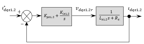
The Figure 8 shows the diagram of the stator current regulation loop (stator 1 and 2):
Figure 8. Diagram of the stator currents regulation
With
$\left\{\begin{array}{l}K_{p s 1}=\frac{L_{s 1}}{T} \\ K_{i s 1}=\frac{R_{s 1}}{T}\end{array} \quad\right.$ and $\quad\left\{\begin{array}{l}K_{p s 2}=\frac{L_{s 2}}{T} \\ K_{i s 2}=\frac{R_{s 2}}{T}\end{array}\right.$ (40)
To have a fast process dynamic, we take $T=\frac{\tau_{r}}{3}$.
The proposed control strategy for a stand-alone variable speed wind energy supply system is performed by Matlab Simulink software, the DSIG parameters are given in Table 1. In this article, we used a nominal value of the charge, which is unable to achieve in the previous work [22, 37, 38], because to charge the battery bank the load must be lower than the nominal power value of the induction machine.
Table 1. DSIG parameters
|
Components |
Rating values |
|
Nominal power |
Pn = 4.5 kW |
|
Power winding resistance |
Rs1 =2.79 Ω |
|
Control winding resistance |
Rs2 =4.65 Ω |
|
Rotor resistance |
Rr = 2.12 Ω |
|
Power winding inductance |
Ls1= 0.0165 H |
|
Control winding inductance |
Ls2=0.0275 H |
|
Rotor inductance |
Lr = 0.006 H |
|
Mutual inductance |
Lm = 0.3672 H |
|
Moment of inertia |
J = 0.0625 kg .m2 |
|
Viscous friction |
f = 0.001 N m. s/rd |
|
Rate speed |
$\Omega_{m}=293 \mathrm{rad} / \mathrm{s}$ |
|
Number of pole pairs |
P=1 |
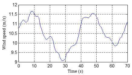
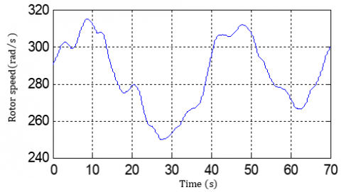
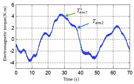
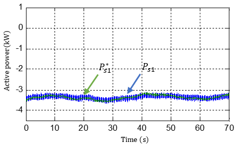
The wind profile is shown in the Figure 9 which will give us the speed profile of the DSIG illustrated in Figure 10, in these conditions, we can see well the regulation made by the control winding through the Figure 11 and Figure 12 which we note respectively that the electromagnetic torque and the active power follow the variation of the wind speed in order to properly balance the power response to compensate the missing power of the stator 1 which provide constant power to the load and to charge the battery bank in the other case. The active power of the stator 1 remains constant and the electromagnetic torque follows the variation of the wind speed shown in Figure 13 and Figure 14 respectively.
Figure 9. Wind speed profil
Figure 10. DSIG rotor speed
Figure 11. Electromagnetic torque of control winding
Figure 12. Active power of control winding
Figure 13. Active power of power winding
Figure 14. Electromagnetic torque of power winding
Figure 15. DC link voltage of power winding
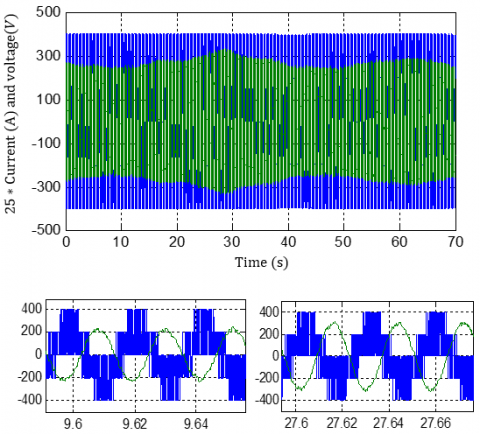
Figure 16. Current and voltage of power winding
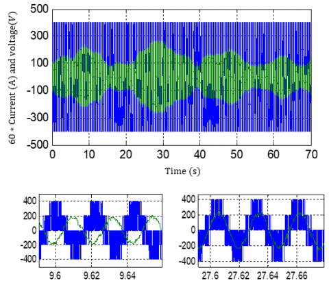
Figure 17. Current and voltage of control winding
The DC-link voltage of the stator 1 was successfully regulated, as shown in Figure 15. despite the step variations in the generator power.
The current and the stator voltage shown in Figure 16 are in phase opposition which means that the stator 1 permanently supplies active power to the load, unlike the stator 2, which we see that are in phase opposition during charging the battery and in phase during restored energy shown in Figure 17.
In this paper, a new power control and DC bus regulation of DSIG with non-identical parameters have been presented. The simulation results of this new power control strategy with a double stator induction machine shows its performance through the continuous bus regulation using flow oriented control and the active power compensation of stator 1 with the power available in the storage battery connected to the stator 2 by calculating the missing power and control it to provide this power as far as possible which is interesting for wind turbines applications in variable speeds.
The study was supported by the renewable energy’s management laboratory of Bejaia university, which I would like to thank its director as well as the researchers who contribute to this work.
|
AC |
Alternating current |
|
Cp |
Turbine power coefficient |
|
$C_{p \max }$ |
Maximum turbine power coefficient |
|
DC |
Direct current |
|
d, q |
Synchronous reference frame index |
|
FOC |
Field oriented control |
|
f |
Viscous bearing friction coefficient |
|
G |
Gear speed ratio |
|
IG |
Induction generator |
|
$I_{d c 1}, I_{d c 2}$ |
Stator rectified currents |
|
$\iota_{q s 1}, l_{q s 2}$ |
Stator quadratic currents |
|
$\boldsymbol{l}_{d s 1}, \boldsymbol{l}_{d s} 2$ |
Stator direct currents |
|
ldr |
Rotor direct currents |
|
lqr |
Rotor quadratic currents |
|
J |
Total moment of inertia |
|
Kp |
Proportional gain |
|
Ki |
Integral gain |
|
Ls1, Ls2 |
Per phase stator leakage-inductance |
|
Lm |
Cyclic mutual inductance |
|
Lr |
Per phase rotor leakage-inductance. |
|
MPPT |
Maximum power point tracking |
|
P |
Number of pole pairs |
|
Ps1, Ps2 |
Active power |
|
Pt |
Turbine power |
|
PWM |
Pulse width modulation |
|
Qs1, Qs2 |
Reactive power |
|
R |
Turbine radius |
|
Rs1, Rs2 |
Per phase stator resistance |
|
Rr |
Per phase rotor resistance |
|
S |
Surface swept by rotor blade |
|
s |
Laplace operator |
|
Tg |
Generator torque |
|
Tt |
Turbine torque |
|
$T_{o p t}^{*}$ |
Optimal torque reference |
|
$T_{e m 1}^{*}, T_{e m 2}^{*}$ |
Electromagnetic torque reference |
|
$v_{d s 1}, v_{d s 2}$ |
Stator direct voltage |
|
$v_{q s 1}, v_{q s 2}$ |
Stator quadratic voltage |
|
vdr |
Rotor direct voltage |
|
vqr |
Rotor quadratic voltage |
|
Vwind |
Wind speed |
|
Greek symbols
|
|
|
$\alpha$ |
Shift angle |
|
$\beta$ |
Pitch angle |
|
$\theta_{r}$ |
Rotor electrical angle |
|
$\theta_{S}$ |
Synchronous reference frame angle |
|
$\lambda$ |
Speed ratio |
|
$\lambda_{o p t}$ |
Optimal speed ratio |
|
$\rho$ |
Air density |
|
$\tau_{r}$ |
Rotor time constant |
|
$\varphi_{d s 1}, \varphi_{d s 2}$ |
Stator direct flux |
|
$\varphi_{q s 1}, \varphi_{q s 2}$ |
Stator quadratic flux |
|
$\varphi_{d r}$ |
Rotor direct flux |
|
$\varphi_{q r}$ |
Rotor quadratic flux |
|
$\varphi_{r}^{*}$ |
Rotor reference flux |
|
$\varphi_{r}$ |
Rotor flux |
|
$\Omega_{m}$ |
Mechanical speed |
|
$\Omega_{t}$ |
Turbine speed |
|
$\omega_{r}$ |
Rotor electrical angular speed |
|
$\omega_{S}$ |
Synchronous reference frame speed |
|
$\omega_{Sl}$ |
Slip speed |
Identification method of PI regulator parameters:
The identification of the PI regulators parameters of the systems whose transfer function is first order, such as:
$H(s)=\frac{1}{a s+b}$ (41)
The transfer function of the PI regulator is given by:Is generally done as follows:
$C(s)=K_{p}+\frac{K_{i}}{s}$ (42)
The diagram representing the regulation loop of a first order control system with unitary return regulated by a PI is given in Figure 18.
Figure 18. First order control system regulated by a PI
The disturbance is neglected in the identification step of the regulator parameters. The open loop transfer function of the control system is:
$T(s)=C(s) H(s)=\frac{K_{p} s+K_{i}}{a s^{2}+b s}$ (43)
In a closed loop, we obtain:
$F(s)=\frac{T(s)}{1+T(s)}=\frac{K_{p} s+K_{i}}{a s^{2}+\left(b+K_{p}\right) s+K_{i}}$ (44)
In order to have the behavior of a first order system whose transfer function is of the form:
$G(s)=\frac{1}{T s+1}$ (45)
We identify (44) and (45) as follows:
$\frac{K_{p} s+K_{i}}{a s^{2}+\left(b+K_{p}\right) s+K_{i}}=\frac{1}{T s+1}$ (46)
which give:
$K_{p} T s^{2}+\left(K_{i} T+K_{p}\right) s+K_{i}=a s^{2}+\left(b+K_{p}\right) s+K_{i}$ (47)
After identification, the PI regulator parameters are given as:
$\left\{\begin{aligned} K_{p} &=\frac{a}{T} \\ K_{i} &=\frac{b}{T} \end{aligned}\right.$ (48)
[1] Hamoud, F., Doumbia, M.L., Cheriti, A. (2016). Performance study of a self-excitation dual stator winding induction generator for renewable distributed generation systems. Smart Grid and Renewable Energy, 7: 197-215. http://dx.doi.org/10.4236/sgre.2016.76016
[2] Lin, W.M., Hong C.M. (2010). Intelligent approach to maximum power point tracking control strategy for variable-speed wind turbine generation system. Energy, 35(6): 2440-2447. https://doi.org/10.1016/j.energy.2010.02.033
[3] Yin, X.X., Jiang, Z.D., Li, P. (2020). Recurrent neural network based adaptive integral sliding mode power maximization control for wind power systems. Renewable Energy, 145: 1149-1157. https://doi.org/10.1016/j.renene.2018.12.098
[4] Benakcha, M., Benalia, L., Tourqui, D.E., Benakcha, A. (2018). Backstepping control of dual stator induction generator used in wind energy conversion system. International Journal of Renewable Energy Research, 8(1): 384-395.
[5] Bedoud, K., Ali-rachedi, M., Bahi, T., Lakel, R. (2015). Adaptive fuzzy gain scheduling of PI controller for control of the wind energy conversion systems. Energy Procedia, 74: 211-225. https://doi.org/10.1016/j.egypro.2015.07.580
[6] Chenna, A., Aouzellag, D., Ghedamsi, K. (2020). Study and control of a pumped storage hydropower system dedicated to renewable energy resources. Journal Européen des Systèmes Automatisés, 53(1): 95-102. https://doi.org/10.18280/jesa.530112
[7] Singh, B., Kasal, G.K. (2008). Solid-state voltage and frequency controller for a stand-alone wind power generating system. IEEE Trans. Power Electronics, 23(3): 1170-1177. https://doi.org/10.1109/TPEL.2008.921190
[8] Wang, D., Ma, W., Xiao, F., Zhang, B., Liu, D., Hu, A. (2005). A novel stand-alone dual stator-winding induction generator with static excitation regulation. IEEE Transactions on Energy Conversion, 20(4): 826-835. https://doi.org/10.1109/TEC.2005.853744
[9] Amimeur, H., Abdessemed, R., Aouzellag, D., Ghedamsi, K. (2012). Sliding mode control of a dual-stator induction for wind energy conversion systems. Electrical Power and Energy Systems, 42(1): 60-70. https://doi.org/10.1016/j.ijepes.2012.03.024
[10] Hadiouche, D., Razik, H., Rezzoug, A. (2004). On the modeling and design of dual-stator windings to minimize circulating harmonic currents for VSI fed AC machines. IEEE Transactions on Industry Applications, 40(2): 506-515. https://doi.org/10.1109/TIA.2004.824511
[11] Yazdani, D., Ali Khajehoddin, S., Bakhshai, A., Joos, G. (2009). Full utilization of the inverter in split-phase drives by means of a dual three-phase space vector classification algorithm. In IEEE Transactions on Industrial Electronics, 56(1): 120-129. https://doi.org/10.1109/TIE.2008.927405
[12] Khlifi, M.A., Ben Slimene, M., Ben Fredj, M., Rhaoulia, H. (2015). Performance evaluation of self-excited DSIG as a stand-alone distributed energy resources. Electrical Engineering, 98(2): 159-167. https://doi.org/10.1007/s00202-015-0349-y
[13] Bu, F., Huang, W., Hu, Y., Shi, K. (2010). Optimal selection of excitation capacitor for 6/3-phase dual stator-winding induction generator with the static excitation controller applied in wind power. Energy Conversion Congress and Exposition (ECCE), 2010 IEEE, pp. 2397-2402. https://doi.org/10.1109/ECCE.2010.5617905
[14] Wang, C., Wang, K., You, X. (2016). Research on synchronized SVPWM strategies under low switching frequency for six-phase VSI-fed asymmetrical dual stator induction machine. in IEEE Transactions on Industrial Electronics, 63(11): 6767-6776. https://doi.org/10.1109/TIE.2016.2585459
[15] Levi, E. (2008). Multiphase electric machines for variable- speed applications. IEEE Transactions on Industrial Electronics, 55(5): 120-128. https://doi.org/10.1109/TIE.2008.918488
[16] Barrero, F., Duran, M.J. (2016). Recent advances in the design, modeling, and control of multiphase machines-part I. IEEE Transactions on Industrial Electronics, 63(1): 449-458. https://doi.org/10.1109/TIE.2015.2447733
[17] Duran, M.J., Barrero, F. (2016). Recent advances in the design, modeling, and control of multiphase machines-Part II. IEEE Trans. Ind. Electron., 63(1): 459-468. https://doi.org/10.1109/TIE.2015.2447733
[18] Amimeur, H., Abdessemed, R., Aouzellag, D., Merabet, E., Hamoudi, F. (2010). A sliding mode control associated to the field-oriented control of dual-stator induction motor drives. Journal of Electrical Engineering, 10(3): 7-12.
[19] Chekkal, S., Lahaçani, N.A., Aouzellag, D., Ghedamsi, K. (2014). Fuzzy logic control strategy of wind generator based on the dual-stator induction generator. International Journal of Electrical Power & Energy Systems, 59: 166-175. https://doi.org/10.1016/j.ijepes.2014.02.005
[20] Marouani, K., Baghli, L., Hadiouche, D., Kheloui, A., Rezzoug, A. (2008). A new PWM strategy based on a 24-sector vector space decomposition for a six-phase VSI-fed dual stator induction motor. IEEE Transactions on Industrial Electronics, 55(5): 1910-1920. https://doi.org/10.1109/TIE.2008.918486
[21] Merabet, E., Abdessemed, R., Amimeur, H., Hamoudi, F. (2007). Field oriented control of a dual star induction machine using fuzzy regulators. In 4th Int. Conf. Computer Integrated Manufacturing.
[22] Tanvir, A.A., Merabet, A. (2020). Artificial neural network and Kalman filter for estimation and control in standalone induction generator wind energy DC microgrid. Energies, 13(7): 1743. https://doi.org/10.3390/en13071743
[23] Krishnasamy, V., Kumaresan, N., Gounden, A. (2011). Operation and closed-loop control of wind-driven stand-alone doubly fed induction generators using a single inverter-battery system. IET Electric Power Applications, 6(3):162-171. https://doi.org/10.1049/iet-epa.2011.0204
[24] Abrahamsen, A.B., Mijatovic, N., Seiler, E., Zirngibl, T., Traeholt, C., Norgard, P.B., Pedersen, N.F., Andersen, N.H., Østergård, J. (2010). Superconducting wind turbine generators. Superconductor Science and Technology, 23(3): 034019. https://doi.org/10.1088/0953-2048/23/3/034019
[25] Navas, M.A.H., Puma, J.L.A., Filho, A.J.S. (2015). Direct torque control for squirrel cage induction generator based on wind energy conversion system with battery energy storage system. 2015 IEEE Workshop on Power Electronics and Power Quality Applications (PEPQA), Bogota, pp. 1-6. https://doi.org/10.1109/PEPQA.2015.7168203
[26] Howlader, A.M., Urasaki, N., Saber, A.Y. (2014). Control strategies for wind-farm-based smart grid system. IEEE Transactions on Industry Applications, 50(5): 3591–3601. https://doi.org/10.1109/tia.2014.2304411
[27] Ghedamsi, K., Aouzellag, D., Berkouk, E.M. (2008). Control of wind generator associated to a flywheel energy storage system. Renew Energy, 33(9): 2145-2156. https://doi.org/10.1016/j.renene.2007.12.009
[28] Poitiers, F., Machmoum, M. (2001). Control of a doubly fed induction generator for wind energy conversion systems. In: GE44-LARGE, Saint Nazaire, France.
[29] Aouzellag, D., Ghedamsi, K., Berkouk, E.M. (2006). Power control of a variable speed wind turbine driving an DFIG. Renewable Energy and Power Quality Journal, Vol. 1. https://doi.org/10.24084/repqj04.220
[30] Hadiouche, D. (2001). Contribution to the study of dual stator induction machines: Modeling, supplying and structure. (in French), Ph.D. dissertation, GREEN, Faculty Sci. Tech. Univ. Henri Poincare-Nancy I, Vandœuvre-lès-Nancy, France.
[31] Singh, G.K., Yadav, K.B., Saini, R.P. (2005). Modeling and analysis of multi-phase (six phase) self-excited induction generator. In Proc. IEEE Conf. ICEMS’2005, pp. 1922-1927. https://doi.org/10.1109/ICEMS.2005.202896
[32] Sadouni, R., Meroufel, A. (2012). Performances comparative study of field oriented control (FOC) and direct torque control (DTC) of dual three phase induction motor (DTPIM). International Journal of Circuits, Systems and Signal Processing, 2(6): 163-170.
[33] Singh, G.K., Nam, K., Lim, S.K. (2005). A simple indirect field-oriented control scheme for multiphase induction machine. IEEE Trans. Ind. Elect., 52(4): 1177-1184. https://doi.org/10.1109/TIE.2005.851593
[34] Beriber, D., Berkouk, E.M., Talha, A., Mahmoudi, M.O. (2004). Study and control two two-level PWM rectifiers-clamping bridge-two three-level NPC VSI cascade Application to double stator induction machine. 35th Annual IEEE Electronics Specialists Conference, Aachen, Germany, pp. 3894-3899. https://doi.org/10.1109/PESC.2004.1355164
[35] Pant, V., Singh, G.K., Singh, S.N. (1999). Modeling of a multi-phase induction machine under fault condition. IEEE International Conference on Power Electronics and Drive Systems, PEDS’99, Hong Kong, pp. 92-97.
[36] Ojo, O., Davidson, I.E. (2000). PWM-VSI inverter-assisted stand-alone dual stator winding induction generator. IEEE Transactions on Industry Applications, 36(6): 1604-1611. https://doi.org/10.1109/28.887212
[37] Ndiaye, A., Kébé, C.M.F., Sambou, V., Ndiaye, P.A. (2014). Development of a charge controller dedicated to the small wind turbine system. Energy and Environment Research, 4(3): 68-77. https://doi.org/10.5539/eer.v4n3p68
[38] Hussein, M.M., Senjyu, T., Orabi, M., Wahab, M.A.A., Hamada, M.M. (2013). Control of a stand-alone variable speed wind energy supply system. Applied Sciences, 3: 437-456. https://doi.org/10.3390/app3020437