Nan Xiao | Yuanyuan Liu* | Xinyue Zhang | Yan Liu
© 2020 IIETA. This article is published by IIETA and is licensed under the CC BY 4.0 license (http://creativecommons.org/licenses/by/4.0/).
OPEN ACCESS
The accuracy of swing angle directly bears on the machining performance of computer numerical control (CNC) machine tools. Any error in the swing angle will greatly affect the machining quality. In actual engineering, it is very important to compensate for the angle error in the machine tool. This paper attempts to design an effective method to compensate for the swing angle error in special-shaped rock turning-milling machining center HTM50200. Firstly, the commonly used swing angles of the tool axle were measured, and fitted into curves through polynomial regression. Based on the fitted curves, the error between the theoretical and actual swing angles was obtained and corrected, and the change law of the angle error was derived. After error compensation, the actual swing angle was measured again for verification. According to the measured results, our error compensation technique greatly enhanced the rotation accuracy of the swing axle, and mitigated the effects of swing angle error on machining accuracy. This research breaks new ground for the development of high-end high-precision rock machining equipment.
five-axis computer numerical control (CNC) machine tool, special-shaped rock, swing angle, error compensation, engraving and milling (EM) head
Computer numerical control (CNC) is the automated control of machining tools by means of a computer. Thanks to technological progress and the application of Internet technology, CNC machine tools have developed into the most basic units in modern manufacturing. Facing the increasingly high accuracy requirements, high-precision, high-intelligence, and networking are the major design trends of CNC machine tools [1].
In recent years, the accuracy improvement of CNC machine tools has become one of the hot topics in the industry of manufacturing equipment. With the transformation and upgrading of manufacturing and rock processing industry, there is a surging demand for special-shaped rocks and rock products (e.g. rock borders and pillars of various sections). As a result, the need for high-end CNC machine tools continues to increase [2].
Five-axis CNC machine tool is the most important processing equipment for parts with complex surfaces. Unlike the traditional three-axis CNC machine tool, five-axis CNC machine tool can process all profiles simultaneously once the workpiece is clamped, eliminating the error of repeated positioning induced by multiple clamping. The advantages of five-axis CNC machine tool include accurate adjustment of tool pose, high cutting efficiency, and fast workpiece installation [3]. However, the accuracy of five-axis CNC machine tool is affected by the swing axle, which is not present in three-axis CNC machine tool, posing a threat to the quality of the processed parts [4].
To ensure the accuracy of machine tools, the key lies in measuring the geometric errors and verifying the position accuracy of each coordinate axis, which is an important means of daily maintenance and fault tracing of machine tools [5]. Based on various testing instruments, many methods have been designed to measure the geometric error of the swing axle. For example, Wang and Guo [6] and He et al. [7] measured the geometric error of turntable with laser tracker and Doppler laser instrument, respectively. But the rotation axle of the machine tool is partly beneath the workbench. The motion accuracy of this part can only be measured and improved, when the machine tool is being assembled. Dassanayake et al. [8] and Zargarbashi and Mayer [9] both measured the geometric error of the swing axle with ball bar. However, the one-dimensional (1D) displacement measured by the ball bar fails to cover the information of many key error sources in the three-dimensional (3D) space. Based on the 1D information, it is difficult to realize automatic and efficient testing of machine tool accuracy. Florussen and Spaan [10], Weikert [11], and Ibaraki et al. [12] used the R-test measuring system to identify the geometric error of the swing axle. The system precision depends on the installation accuracy of relevant instruments on the machine tool [13]. If the axial vectors of the measurement coordinate system are not parallel to those of the machine tool coordinate system, the measured data will be so inaccurate as to distort the identification result.
Although many new instruments have been developed to measure the geometric error of the swing axle in five-axis CNC machine tool, these advanced testing instruments are not available in most industrial scenes [14]. It is very meaningful to design a practical geometric error measuring method for the swing axle in five-axis CNC machine tool based on conventional instruments.
Compared with the instrument-based measuring method, the cutting test piece can accurately reflect the geometric accuracy of the swing axle on CNC machine tools. For instance, Jiang et al. [15] analyzed the performance and identified the error of a CNC machine tool based on S-shaped test pieces. However, the relevant research findings have not been widely applied in engineering.
In China, the positioning accuracy/error of swing angle in five-axis machining centers is measured/compensated for, using expensive laser measuring systems. There is not yet a n automated, easy-to-use, low-cost measuring system. The common measuring instruments include 360-tooth division plate on standard turntable, laser interferometer etc. [16]. Among them, the laser interferometer can accurately measure straight lines and small swing angles, but performs poorly if the swing angle is equal to or greater than positive and negative 90°. The other methods are too complicated for automatic measurement [17].
In actual machining, the rotation center of the tool is far from the tool center. Any error in the swing angle of tool axle will greatly affect the spatial position of the tool tip. Focusing on special-shaped rock turning-milling machining center HTM50200, this paper measures the commonly used swing angles of the tool axle, and derives the change law of the angle error of the rotation axle in the machining center [18]. Specifically, the measured data were fitted into curves through polynomial regression. Based on the fitted curves, the error between the theoretical and actual swing angles was obtained, and compensated for. After the compensation, the actual swing angle was measured again. The measured results show that the error compensation effectively improved the rotation accuracy of the swing axle, reducing the effects of swing angle error on machining accuracy [19].
The remainder of this paper is organized as follows: Section 2 briefly introduces the special-shaped rock turning-milling machining center HTM50200; Section 3 proposes our error compensation technique for the swing angle of the engraving and milling (EM) head; Section 4 explains the postprocessing functions of HTM50200; Section 5 puts forward the conclusions.
The five-axis rock machining center can engrave and process large rocks, for its gantry-type frame structure has a large workspace, high stability, and strong rigidity [20]. Compared with other CNC machining techniques, five-axis CNC machine tool boasts a wide applicable scope, and excellent performance in processing parts with complex surfaces. The tool can produce high-quality parts with a high efficiency [21].
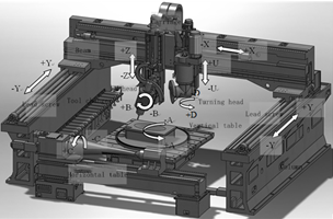
As shown in Figure 1, the special-shaped rock turning-milling machining center HTM50200 contains two five-axis modules and supports eight-axis machining of complex special-shaped rocks. There are four functional modules in the machining center, including a three-axis machining module, two four-axis machining modules (vertical four-axis and horizontal four-axis), two five-axis machining modules (vertical five-axis and horizontal five-axis), and a turning module [22].
The turning module works differently from metal turning. During the turning of metal parts, the workpiece is rotated at a certain speed, while the tool is fixed on the holder; the holder interpolates two coordinates on the turning plane to obtain the outer contour of the workpiece. The turning of special-shaped rocks adopts a different technique from metal turning: the tool is a diamond saw blade rotating around the tool axis; when the contour of the special-shape rock is subject to two-coordinate interpolation on the XOZ plane, the tool and the workpiece move relative to each other at a certain speed. The workpiece-tool speed ratio is smaller than 1, which varies with the properties of the rock [23].
Figure 1. The structure of HTM50200
3.1 Cause and compensation method for swing angle error of EM head
With the development of numerical control systems and computer technology, numerical control systems provide more and more software compensation functions to maximize the accuracy of CNC machine tools [24].
During the processing of complex surfaces, HTM50200’s swing angle error mainly comes from the inherent error of the mechanical structure, because the rotation of the EM head is driven by the worm gear of the actuator. Besides, once the tool is installed, the sheer length (500mm) of the swing axle of the EM head will lead to the following situation: Due to the long distance between the rotation center of the swing axle and the tool tip, a small rotation error will cause the tool tip to deviate greatly from the theoretical position.
To reduce the effect of swing angle error on machining accuracy, the swing angles of the tool axle were fitted into curves through polynomial regression, and the actual swing angle of the EM head was compared with the theoretical swing angle, revealing the change law of the error with swing angle. Based on the change law, the swing angle error was compensated for to ensure the accuracy of machining [25].
3.2 Simplified model of EM head motions
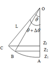
Before theorizing the change law of swing angle error, the actual motions of the EM head were simplified into a geometric model (Figure 2).
Let θt, θa, and Δθ be theoretical value, actual value, and error of the swing angle of tool axle, respectively, OA be the vertical position of the swing axle, OB be the position of the swing axle after rotating by the theoretical swing angle, and OC be the actual position of the tool tip under the effect of the error of worm gear operation. It is assumed that $h=Z_{1}-Z_{2}, h^{\prime}=Z_{1}-Z_{3},$ and $\Delta Z=Z_{2}-Z_{3}$.
Figure 2. The simplified model of EM head motions
In actual measurement, the tool is a ball-nose cutter with a diameter of 8mm and a length of 700mm. The distance L from the cutter center to the rotation center of the EM head is 577.11mm. Then, the swing angle error and its change law were indirectly derived from the difference between the theoretical and actual vertical positions of the tool tip.
The indirect derivation is not so accurate as professional measuring instruments. But the accuracy is sufficient to reveal the change law of swing angle error. According to the simplified model in Figure 2, the following equation holds:
$L(1-\cos (\theta))=h$ (1)
$L(1-\cos (\theta+\Delta \theta))=h^{\prime}$ (2)
From formulas (1) and (2), we have:
$L(\cos (\theta)-\cos (\theta+\Delta \theta))=\Delta Z$ (3)
$\cos (\theta+\Delta \theta)=\cos (\theta)-\Delta Z / L$ (4)
Then, the relationship between swing angle error and vertical position of tool tip can be obtained as:
$\Delta \theta=a \cos (\cos (\theta)-\Delta Z / L)-\theta$ (5)
Firstly, the change law of h with swing angle θ was observed. The common range ($0^{\circ} \sim 40^{\circ}$) of swing angle in actual processing was divided into $1^{\circ}$ intervals. Then, the following can be derived from formula (1):
$d h=L \sin (\theta) d \theta$ (6)
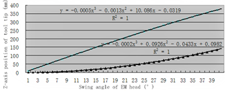
Figure 3. The change law of the speed for vertical position increment of tool tip with the swing angle of EM head
Then, the change law of h with swing angle θ, that is, the change law of the speed for vertical position increment of tool tip with the swing angle of EM head, can be plotted as Figure 3.
As shown in Figure 3, the Z-axis position of tool tip increased with the swing angle of EM head, and the increasing rate grew over time. This is the theoretical change law of the Z-axis position of tool tip with swing angle.
3.3 Swing angle error measurement and processing
To obtain the change law of actual swing angle error with swing angle, the actual position Z3 of tool tip in the space was measured, with the vertical position Z1 as the benchmark, and compared with the theoretical angle Z2. Moreover, the measured data were fitted into curves through polynomial regression, and analyzed to obtain the said change law.
During the swing angle measurement, the actual deviation of swing angle was obtained through geometric calculation based on the spatial coordinates of the center of the reference sphere in contact with the reference plane [26]. The compensation value was preset through software programming or CNC system of the machine tool [27]. Some measured data are listed in Table 1. Every item is the average of repeated measurements.
The measured data were processed and simplified by formula (3) to reveal the change law of Z-axis position error of tool tip with swing angle and that of actual swing angle error with swing angle. Some of the processed data are presented in Table 2.
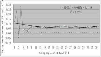
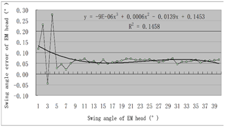
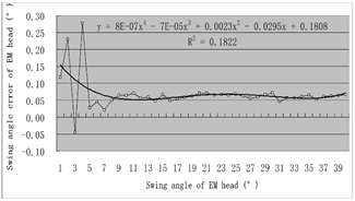
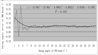
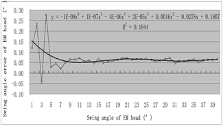
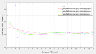
The position errors of tool tip in Table 2 were fitted into curves through polynomial regression, with x as the swing angle and y as swing angle error. For simplicity, it is necessary to determine the best order of the polynomial [28]. The swing angle error curves fitted by polynomial of the second, third, fourth, fifth, and sixth orders are presented in Figures 4-8, respectively. The fitted curves by different polynomials are compared in Figure 9. Note that the dotted lines are measured data, and the curves are fitted.
As shown in Figures 4-8, not all the many data points were passed through by the fitted curves. Theoretically, the fitting accuracy should increase with the order of the polynomial. It can be seen from Figure 9 that, the fitting accuracies of second and third-order polynomials were not as good as those of fourth, fifth, and sixth-order polynomials. However, the curves fitted by latter three polynomials were of similar accuracy.
In Figures 4-8, the chi-square statistic (R2) was 0.0953, 0.1458, 0.1822, 0.1835, and 0.1844, respectively, indicating that the fitted curves can explain 9.53%, 14.58%, 18.22%, 18.35%, and 18.44% of the measured data, respectively. Judging by the change trend of this statistic, the curve fitted by the fourth-order polynomial was selected to demonstrate the change law of swing angle error with swing angle.
In addition, the fitted curves show that the swing angle error y of the EM head fluctuated greatly near the vertical position. With the growing swing angle x, the error basically remained on the same level and tended to be stable; the reference line of the fitted curve of swing angle error was about +0.05° above the zero baseline, and the error changed between -0.05° and 0.3°. After fully analyzing the fitted curves, the change law of swing angle error with swing angle can be expressed by the following polynomial:
$y=-8 \times 10^{-7} x^{4}-7 \times 10^{-5} x^{3}+2.3 \times 10^{-3} x^{2}-2.95 \times 10^{-2} x+0.1808$
Table 1. The measured data (unit: mm)
|
θ |
cos(θ) |
h=L(1-cos(θ)) |
dh/dθ |
Z1 |
Z2 |
Z3 |
|
1 |
0.999848 |
0.087897 |
10.071958 |
-170.99 |
-171.077897 |
-171.1000 |
|
2 |
0.999391 |
0.351560 |
20.140849 |
-170.99 |
-171.341560 |
-171.4275 |
|
3 |
0.998630 |
0.790909 |
30.203604 |
-170.99 |
-171.780909 |
-171.7575 |
|
4 |
0.997564 |
1.405811 |
40.257159 |
-170.99 |
-172.395811 |
-172.5975 |
|
5 |
0.996195 |
2.196078 |
50.298451 |
-170.99 |
-173.186078 |
-173.2100 |
|
6 |
0.994522 |
3.161469 |
60.324421 |
-170.99 |
-174.151469 |
-174.2000 |
|
7 |
0.992546 |
4.301690 |
70.332017 |
-170.99 |
-175.291690 |
-175.3175 |
|
8 |
0.990268 |
5.616395 |
80.318188 |
-170.99 |
-176.606395 |
-176.6775 |
|
9 |
0.987688 |
7.105182 |
90.279894 |
-170.99 |
-178.095182 |
-178.1975 |
|
10 |
0.984808 |
8.767598 |
100.214100 |
-170.99 |
-179.757598 |
-179.8700 |
|
11 |
0.981627 |
10.603136 |
110.117779 |
-170.99 |
-181.593136 |
-181.7300 |
|
12 |
0.978148 |
12.611238 |
119.987916 |
-170.99 |
-183.601238 |
-183.7175 |
|
13 |
0.974370 |
14.791292 |
129.821503 |
-170.99 |
-185.781292 |
-185.9175 |
|
14 |
0.970296 |
17.142633 |
139.615545 |
-170.99 |
-188.132633 |
-188.2475 |
|
15 |
0.965926 |
19.664546 |
149.367059 |
-170.99 |
-190.654546 |
-190.8300 |
|
16 |
0.961262 |
22.356263 |
159.073074 |
-170.99 |
-193.346263 |
-193.4800 |
|
17 |
0.956305 |
25.216962 |
168.730635 |
-170.99 |
-196.206962 |
-196.3675 |
|
18 |
0.951057 |
28.245774 |
178.336798 |
-170.99 |
-199.235774 |
-199.4175 |
|
19 |
0.945519 |
31.441775 |
187.888638 |
-170.99 |
-202.431775 |
-202.6375 |
|
20 |
0.939693 |
34.803992 |
197.383245 |
-170.99 |
-205.793992 |
-206.0400 |
|
21 |
0.933580 |
38.331400 |
206.817727 |
-170.99 |
-209.321400 |
-209.5800 |
|
22 |
0.927184 |
42.022926 |
216.189211 |
-170.99 |
-213.012926 |
-213.2575 |
|
23 |
0.920505 |
45.877444 |
225.494842 |
-170.99 |
-216.867444 |
-217.1275 |
|
24 |
0.913545 |
49.893781 |
234.731784 |
-170.99 |
-220.883781 |
-221.1525 |
|
25 |
0.906308 |
54.070713 |
243.897225 |
-170.99 |
-225.060713 |
-225.3500 |
|
26 |
0.898794 |
58.406968 |
252.988373 |
-170.99 |
-229.396968 |
-229.6755 |
|
27 |
0.891007 |
62.901225 |
262.002457 |
-170.99 |
-233.891225 |
-234.1475 |
|
28 |
0.882948 |
67.552115 |
270.936734 |
-170.99 |
-238.542115 |
-238.8275 |
|
29 |
0.874620 |
72.358221 |
279.788480 |
-170.99 |
-243.348221 |
-243.6725 |
|
30 |
0.866025 |
77.318079 |
288.555000 |
-170.99 |
-248.308079 |
-248.6700 |
|
31 |
0.857167 |
82.430179 |
297.233623 |
-170.99 |
-253.420179 |
-253.6575 |
|
32 |
0.848048 |
87.692963 |
305.821707 |
-170.99 |
-258.682963 |
-258.9875 |
|
33 |
0.838671 |
93.104829 |
314.316633 |
-170.99 |
-264.094829 |
-264.4075 |
|
34 |
0.829038 |
98.664127 |
322.715817 |
-170.99 |
-269.654127 |
-270.0025 |
|
35 |
0.819152 |
104.369164 |
331.016697 |
-170.99 |
-275.359164 |
-275.7400 |
|
36 |
0.809017 |
110.218202 |
339.216747 |
-170.99 |
-281.208202 |
-281.5175 |
|
37 |
0.798636 |
116.209461 |
347.313468 |
-170.99 |
-287.199461 |
-287.5675 |
|
38 |
0.788011 |
122.341114 |
355.304394 |
-170.99 |
-293.331114 |
-293.7175 |
|
39 |
0.777146 |
128.611294 |
363.187091 |
-170.99 |
-299.601294 |
-300.0025 |
|
40 |
0.766044 |
135.018091 |
370.959157 |
-170.99 |
-306.008091 |
-306.4400 |
Table 2. The processed data (unit: mm)
|
Z1-Z3 |
Z1-Z2 |
Z2-Z3 |
△θ=acos (cosθ-△Z/L)-θ |
|
0.110000 |
0.087897 |
0.022103 |
0.118695 |
|
0.437500 |
0.351560 |
0.085940 |
0.231130 |
|
0.767500 |
0.790909 |
-0.023409 |
-0.044740 |
|
1.607500 |
1.405811 |
0.201689 |
0.277447 |
|
2.220000 |
2.196078 |
0.023922 |
0.027177 |
|
3.210000 |
3.161469 |
0.048531 |
0.045919 |
|
4.327500 |
4.301690 |
0.025810 |
0.020994 |
|
5.687500 |
5.616395 |
0.071105 |
0.050565 |
|
7.207500 |
7.105182 |
0.102318 |
0.064705 |
|
8.880000 |
8.767598 |
0.112402 |
0.064061 |
|
10.740000 |
10.603136 |
0.136864 |
0.070986 |
|
12.727500 |
12.611238 |
0.116262 |
0.055391 |
|
14.927500 |
14.791292 |
0.136208 |
0.059978 |
|
17.257500 |
17.142633 |
0.114867 |
0.047062 |
|
19.840000 |
19.664546 |
0.175454 |
0.067155 |
|
22.490000 |
22.356263 |
0.133737 |
0.048100 |
|
25.377500 |
25.216962 |
0.160538 |
0.054429 |
|
28.427500 |
28.245774 |
0.181726 |
0.058293 |
|
31.647500 |
31.441775 |
0.205725 |
0.062636 |
|
35.050000 |
34.803992 |
0.246008 |
0.071289 |
|
38.590000 |
38.331400 |
0.258600 |
0.071525 |
|
42.267500 |
42.022926 |
0.244574 |
0.064728 |
|
46.137500 |
45.877444 |
0.260056 |
0.065988 |
|
50.162500 |
49.893781 |
0.268719 |
0.065508 |
|
54.360000 |
54.070713 |
0.289287 |
0.067872 |
|
58.685500 |
58.406968 |
0.278532 |
0.063010 |
|
63.157500 |
62.901225 |
0.256275 |
0.055990 |
|
67.837500 |
67.552115 |
0.285385 |
0.060292 |
|
72.682500 |
72.358221 |
0.324279 |
0.066337 |
|
77.680000 |
77.318079 |
0.361921 |
0.071785 |
|
82.667500 |
82.430179 |
0.237321 |
0.045716 |
|
87.997500 |
87.692963 |
0.304537 |
0.057010 |
|
93.417500 |
93.104829 |
0.312671 |
0.056952 |
|
99.012500 |
98.664127 |
0.348373 |
0.061802 |
|
104.750000 |
104.369164 |
0.380836 |
0.065865 |
|
110.527500 |
110.218202 |
0.309298 |
0.052210 |
|
116.577500 |
116.209461 |
0.368039 |
0.060672 |
|
122.727500 |
122.341114 |
0.386386 |
0.062265 |
|
129.012500 |
128.611294 |
0.401206 |
0.063250 |
|
135.450000 |
135.018091 |
0.431909 |
0.066663 |
Figure 4. The swing angle error fitted by second-order polynomial
Figure 5. The swing angle error fitted by third-order polynomial
Figure 6. The swing angle error fitted by fourth-order polynomial
Figure 7. The swing angle error fitted by fifth-order polynomial
Figure 8. The swing angle error fitted by sixth-order polynomial
Figure 9. The swing angle errors fitted by different polynomials
To conform to the expression of the angle and angle error, $y=\Delta \theta, x=\theta$ were substituted into the above formula:
$\Delta \theta=-8 \times 10^{-7} \theta^{4}-7 \times 10^{-5} \theta^{3}+2.3 \times 10^{-3} \theta^{2}-2.95 \times 10^{-2} \theta+0.1808$
Finally, the actual swing angle can be obtained by:
$\theta_{a}=\theta_{t}+\Delta \theta$ (7)
3.4 Change law of swing angle error after compensation
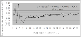
After the swing angle error was compensated for by formula (7), the vertical error was measured again in the range of 0°~40° at an interval of 1°. Based on the measured data, the swing angle error after compensation (as shown in Figure 9) was calculated by formula (5).
As shown in Figure 10, the compensation greatly mitigated the error in swing angle. The baseline of the fluctuating fitted curve coincided with the zero baseline, and the range of the error obviously narrowed to -0.06°~0.09°. Therefore, the error compensation reduces the influence of swing angle error on machining accuracy, and improves the quality of the machined parts.
Figure 10. The post-compensation swing angle error fitted through polynomial regression
The postprocessing functions of HTM50200 mainly include: (1) Processing cutter location source files (CLSFs) from different sources; (2) Setting postprocessing parameters; (3) Postprocessing algorithm judgement; (4) Tool length compensation; (5) Rotation tool center point (RTCP); (6) Data conversion; (7) Nonlinear error check and processing; (8) Feed speed check and processing; (9) Data display and storage; (10) Other functions.
The postprocessing algorithm judgment selects the most suitable angle planning algorithm according to the quadrant of the tool axle vector, a kind of tool position information. During postprocessing, the tool position information in the tool position file is read segment by segment, followed by coordinate conversion, identifiers and auxiliary commands processing, and format conversion [29]. The reading and processing continued until all the segments of the tool position file have been read. In the end, the numerical control program is displayed and stored in the numerical control program library.
Then, the tool path of a 3D rock sculpture was programmed on computer-aided design/computer-aided manufacturing (CAD/CAM) software, according to our polynomial regression method. The programmed path was adopted for simulation and actual machining [30]. Then, the simulated results were compared with the actual results, proving that our method is feasible and correct.
Due to the sheer length of the swing axle of the EM head, a small error in the swing axle will cause the tool tip to deviate greatly from the theoretical position, which undermines the machining accuracy of actual parts. Hence, the swing angle of the axle was measured, revealing the significant impact of swing angle error on machining effect. After the error was compensated for, the actual swing angle error was reduced by over 50% from -0.05°~0.3° to -0.06°~0.09°. This means the error compensation greatly mitigates the negative impact of swing angle error on machining accuracy. Finally, the proposed polynomial regression method was proved correct through the machining of a 3D sculpture.
This work was supported by Liaoning Science and Technology Research Project (Grant No.: 20180550827).
[1] Zhang, Q. (2020). Reliability control technology of NC machine tool assembly based on meta-motion. Equipment Management and Maintenance, 2020(2): 141-143.
[2] Zhao, D.H. (2019). Basic research on special-shaped stone sawing and milling composite processing technology and equipment technology. Dalian University of Technology, 2019.
[3] Li, J., Xie, F.G., Liu, X.J., Mei, B., Dong, Z.Y. (2017). Analysis on the research status of volumetric positioning accuracy improvement methods for five-axis NC machine Tools. Journal of Mechanical Engineering, 53(7): 113-128. https://doi.org/10.3901/JME.2017.07.113
[4] Jiang, Z., Ding, J.X., Du, L., Li, Q.C., Song, Z.Y. (2017). A measuring and optimizing method of five-axis linkage accuracy of CNC machine tools. Manufacturing Technology and Machine Tool, 2017(4): 92-96. https://doi.org/10.19287/j.cnki.1005-2402.2017.04.016
[5] Wang, L.P., Zhang, S.Z., Wang, D. (2020). Geometric error measurement and accuracy verification of the swing head of a five-axis CNC machine tool with a single swing angle. Journal of Tsinghua University (Science and Technology), 60(4): 292-298. http://jst.tsinghuajournals.com/EN/Y2020/V60/I4/292
[6] Wang, J.D., Guo, J.J. (2012). Research on volumetric error compensation for NC machine tool based on laser tracker measurement. Science China Technological Sciences, 55(11): 3000-3009. https://doi.org/10.1007/s11431-012-4959-6
[7] He, Z.Y., Fu, J.Z., Zhang, L.C., Yao, X.H. (2015). A new error measurement method to identify all six error parameters of a rotational axis of a machine tool. International Journal of Machine Tools and Manufacture, 88: 1-8. https://doi.org/10.1016/j.ijmachtools.2014.07.009
[8] Dassanayake, K.M.M., Tsutsumi, M., Saito, A. (2006). A strategy for identifying static deviations in universal spindle head type multi-axis machining centers. International Journal of Machine Tools & Manufacture, 46(10): 1097-1106. https://doi.org/10.1016/j.ijmachtools.2005.08.010
[9] Zargarbashi, S.H.H., Mayer, J.R.R. (2006). Assessment of machine tool trunnion axis motion error, using magnetic double ball bar. International Journal of Machine Tools and Manufacture, 46(14): 1823-1834. https://doi.org/10.1016/j.ijmachtools.2005.11.010
[10] Florussen, G.H.J., Spaan, H.A.M. (2012). Dynamic R-test for rotary tables on 5-Axes machine tools. Procedia CIRP, 1: 536-539. https://doi.org/10.1016/j.procir.2012.04.095
[11] Waikert, S. (2004). R-Test, a new device for accuracy measurements on five axis machine tools. CIRP Annal -Manufacturing Technology, 53(1): 429-432. https://doi.org/10.1016/S0007-8506(07)60732-X
[12] Ibaraki, S., Oyama, C., Otsubo, H. (2010). Construction of an error map of rotary axes on a five-axis machining center by static R-test. International Journal of Machine Tools and Manufacture, 51(3): 190-200. https://doi.org/10.1016/j.ijmachtools.2010.11.011
[13] Xu, M., Wang, H. (2019). Precision testing method of five-axis NC machine tool based on ‘S’ specimen cutting. The Journal of Engineering, 2019(23): 8733-8736. https://doi.org/10.1049/joe.2018.9094
[14] Jiang, Z., Ding, J.X., Song, Z.Y., Du, L., Wang, W. (2016). Modeling and simulation of surface morphology abnormality of ‘S’ test piece machined by five-axis CNC machine tool. The International Journal of Advanced Manufacturing Technology, 85(9-12): 2745-2759. https://doi.org/10.1007/s00170-015-8079-x
[15] Chen, D., Zhang, S., Pan, R., Fan, J. (2018). An identifying method with considering coupling relationship of geometric errors parameters of machine tools. Journal of Manufacturing Processes, 36: 535-549. https://doi.org/10.1016/j.jmapro.2018.10.019
[16] Liu, Y., Zhang, H., Wang, X. (2017). Analysis on influence of perpendicularity error of five axis NC machine tool error modeling accuracy and complexity. Procedia Engineering, 174: 557-565. https://doi.org/10.1016/j.proeng.2017.01.187
[17] Jiang, Z., Ding, J.X., Wang, W., Deng, M., Du, L., Song, Z.Y. (2016). Tracing the source of the dynamic error for five-axis CNC machine tool based on RTCP. Journal of Mechanical Engineering, 52(7): 187-195. https://doi.org/10.3901/JME.2016.07.187
[18] Ibaraki, S., Yoshida, I., Asano, T. (2019). A machining test to identify rotary axis geometric errors on a five-axis machine tool with a swiveling rotary table for turning operations. Precision Engineering, 55: 22-32. https://doi.org/10.1016/j.precisioneng.2018.08.003
[19] Chen, Y., Tang, H., Tang, Q., Zhang, A., Chen, D., Li, K. (2018). Machining error decomposition and compensation of complicated surfaces by EMD method. Measurement, 116: 341-349. https://doi.org/10.1016/j.measurement.2017.11.027
[20] Guan, X.D. (2017). Kinematics research and processing experiment of five-axis stone processing center. Xiamen University, 2017.
[21] Zhu, Z., Peng, F., Yan, R., Li, Z., Wu, J., Tang, X., Chen, C. (2020). Influence mechanism of machining angles on force induced error and their selection in five axis bullnose end milling. Chinese Journal of Aeronautics. https://doi.org/10.1016/j.cja.2019.12.019
[22] Rao, L.W. (2012). Study on dynamic characteristics of HTM50200 special-shaped stone processing center. Shenyang Jianzhu University, 2012.
[23] Hou, Y., Zhang, D., Mei, J., Zhang, Y., Luo, M. (2019). Geometric modelling of thin-walled blade based on compensation method of machining error and design intent. Journal of Manufacturing Processes, 44: 327-336. https://doi.org/10.1016/j.jmapro.2019.06.012
[24] Aguado, S., Samper, D., Santolaria, J., Aguilar, J.J. (2014). Volumetric verification of multiaxis machine tool using laser tracker. The Scientific World Journal, 2014: Article ID 959510. https://doi.org/10.1016/j.proeng.2013.08.189
[25] Uddin, M.S., Ibaraki, S., Matsubara, A., Matsushita, T. (2009). Prediction and compensation of machining geometric errors of five-axis machining centers with kinematic errors. Precision Engineering, 33(2): 194-201. https://doi.org/10.1016/j.precisioneng.2008.06.001
[26] Dassanayake, K.M., Tsutsumi, M., Saito, A. (2006). A strategy for identifying static deviations in universal spindle head type multi-axis machining centers. International Journal of Machine Tools and Manufacture, 46(10): 1097-1106. https://doi.org/10.1016/j.ijmachtools.2005.08.010
[27] Sato, R., Shirase, K. (2018). Geometric error compensation of five-axis machining centers based on on-machine workpiece measurement. International Journal of Automation Technology, 12(2): 230-237. https://doi.org/10.20965/ijat.2018.p0230
[28] Wang, Z., Wang, D., Wu, Y., Dong, H., Yu, S. (2017). Error calibration of controlled rotary pairs in five-axis machining centers based on the mechanism model and kinematic invariants. International Journal of Machine Tools and Manufacture, 120: 1-11. https://doi.org/10.1016/j.ijmachtools.2017.04.011
[29] Li, Z.Z., Sato, R., Shirase, K., Ihara, Y., Milutinovic, D.S. (2019). Sensitivity analysis of relationship between error motions and machined shape errors in five-axis machining center - Peripheral milling using square-end mill as test case. Precision Engineering, 60: 28-41. https://doi.org/10.1016/j.precisioneng.2019.07.006
[30] Gomez, J.L., Khelf, I., Bourdon, A., Hugo, A., Didier, R. (2019). Angular modeling of a rotating machine in non-stationary conditions: Application to monitoring bearing defects of wind turbines with instantaneous angular speed. Mechanism and Machine Theory, 136: 27-51. https://doi.org/10.1016/j.mechmachtheory.2019.01.028