Sudirman Syam* | Sri Kurniati | Ruslan Ramang
© 2020 IIETA. This article is published by IIETA and is licensed under the CC BY 4.0 license (http://creativecommons.org/licenses/by/4.0/).
OPEN ACCESS
This experimental study examines the characteristics and performance of axial magnetic gear by using a variation of the rectangular neodymium-iron-boron (NdFeB) magnetic layer which is assembled on an acrylic disc. The aim is to reduce magnetic reluctance which can increase torque and facilitate the manufacture of magnetic gear. In addition, it can reduce the use of NdFeB permanent magnets instead of sectoral magnets. An appropriate method for predicting the transmitted torque produced by axial magnetic gears with four rectangular magnetic layers is demonstrated using the output power approach. The results show that the performance of axial magnetic-gear with 4 layers tends to be similar to the performance of a direct drive. Tests on the 2400 rpm rotation with the loading of 200, 300 and 400 ohms respectively showed a maximum torque of 2.24 (Nm) 10-3, 1.56 (Nm) 10-3, and 1.1 (Nm). The results of this paper appear to be useful for the development of axial magnetic-gear industrial applications.
DC motor, permanent magnet, torque
In recent years researchers have developed several models to improve the performance of magnetic gear using a pair of magnets or multi-pole [1, 2]. Generally, a magnetic gear transmission is understood to consist of motion or the transfer of torque through non-contacted gear using a driving gear wheel and a driven gear wheel. The principle of conversion of magnetic gear replaces the slot of the mechanical gear tooth to an iron core by using the north-pole (N) and south-pole (S) of the magnet. Magnetic gears are an alternative technology that may offer significant advantages such as, reduced maintenance and improved reliability, inherent overload protection, no mechanical loss, no mechanical fatigue, high efficiency, and physical isolation between input and output shafts [3-8]. In addition, slip and break away from the system when the overload compared with conventional gear when stopping or braking which could damage the machines [9].
There are several magnetic gear types has been introduced by previous researchers. These magnetic gear types consist of a permanent magnet rotor that guides the magnetic flux in iron segments. The other is the output rotor which is driven by this altering flux of the magnetic gear. Gear types are also found in many different configurations. Some of these configurations have the parallel axis and other configurations will transform rotational motion into linear motion. Li et al. [10] proposed a new transmission type using an involute SmCo magnetic gear. In 1993 and 1994, the magnetic worm gear and magnetic skew gear was also developed, respectively [11, 12]. However, both of them have the demerits of complexity and poor torque density.
Due order to avoid the complicated structure of magnetic worm and skew gears, Ikuta et al. [13] have proposed the simple parallel-axis magnetic gears which include two basic topologies: axial coupling and radial coupling. These magnetic gears can be categorized into the category of magnetic gears with closely spaced magnets. This gear type has typically a magnetic interaction in between magnets on two or more axes. The technology is with the two magnetic gear wheels covered with magnets on the surfaces. These magnets interact with each other and they create a driving force on drive magnet wheel. However, although, topology parallel-axis magnetic gear is very simple, but has not been widely used in industrial applications, because it has a low torque density [14]. The application of plastic bonded magnets for gears developed in recent years is an attractive alternative, and the trends are to use them in constructing such devices. They are low cost and do not present fragility in the manufacturing process. Preparation techniques and performance characteristics for the no-load and loaded operation of a magnetic gear system made of the Nd2Fe l4B plastic bonded magnet were reported by Tsamakis et al. [15].
On the other hand, to increase the torque of the magnetic gear, we focused the use of rare-earth permanent magnets of high energy, high remanence, and high coercivity such as neodymium-iron-boron (NdFeB) and samarium-cobalt (SmCo), which was found in 1980 [16, 17]. NdFeB magnet types have high performance compared with other magnets, the attention of researchers to examine the magnetic gear increases performances. In general, sector-shaped magnets were applied in magnetic gear fabrication, therefore it requires sufficient NdFeB magnetic material such as a parallel-axis magnetic gear [13, 18-20], radial magnetic gear [21-23], permanent magnetic spur gear [24], and magnetic planetary gearbox [25]. In addition, there are inherent problems such as price considered expensive and suffer from a shortage of supply. Therefore, a rectangular permanent magnet that can replace sector-shaped magnets in the manufacture of magnetic gears is an appropriate consideration. According to the paper [26], compared with the sector-shaped magnets, they have the merit of low cost due to available dimensional materials. From the geometry point of view, rectangular magnets have the advantages of standard product specifications, low manufacturing cost, and easy magnetization [27].
The purpose of this paper is to conduct experimental of the transmitted torque of a proposed axial magnetic gear with a variation of the rectangular magnet layer. According to the work [28], the use of rectangular magnets arranged in layers is the same as arranging magnetic circuits in parallel. By applying a magnetic circuit analysis approach, an increase in magnetic flux can be achieved by engineering rectangular permanent magnet arrangements in parallel (in layers). To perform magnetic circuit analysis, the electric circuit approach can be used. The resistance (R) and reluctance (Â) are inversely proportional to the area, indicating that the increased surface area will result in a reduction in value and will increase the desired result in the form of current and flux. Compared to the work [13], special attention is given to the application of rectangular magnets to reduce the NdFeB magnetic material used in axial magnetic gears. Unlike radial topology, axial magnetic gear does not require magnetic lengths in the magnetic flux region. They require an axially strong magnetic flux. Different topologies with 1-4 layers of permanent magnet mounted on acrylic discs are tested at 0-2400 rpm. To study the accuracy of the proposed axial magnetic-gear for different load conditions, measurement data obtained between axial magnetic gear and direct drive are compared.
2.1 Structure and design concept
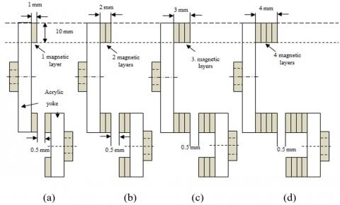
Rectangular magnets with a size of 10mm ´ 20mm ´ 1mm were chosen for fabricating magnetic gears. For this configuration, we want to study the performance of gear when using a disc made of acrylic to reduce magnetic materials. Figure 1 shows a configuration of a magnetic gear that uses disc made of acrylic. Each pair of magnetic poles installed a number of magnetic layers were made of rectangular magnets with a thickness of 1.5 mm. The air gap distance between the disc was adjusted to 0.5 mm. A distance of 0.5 mm between two magnets gear is the most ideal for transferring high torque rotation [29, 30]. The torque decreases with air-gap thickness increase. When the air-gap thickness is small, torque decline with the air-gap thickness increases rapidly. Then, when the air-gap thickness increases to a certain degree, the torque decrease rate will slow down, the effect of the air-gap thickness becomes smaller and smaller. For the experimental variations, we have manufactured four prototypes of axial magnet couplings by using the NdFeB magnet layer that is glued on acrylic discs.
Figure 1. Geometric parameters of the proposed magnetic gear set
Figure 2. Model variation of the studied axial magnetic gear: (a) 1 layer, (b) 2 layers, (c) 3 layers, (d) 4 layers
Table 1. Specifications of a magnetic gear set shown in Figure 1
|
Symbol |
Quantity |
Value |
|
R1d |
Inner radius, drive magnets (mm) |
40 |
|
R2d |
Outer radius of the acrylic discs, drive magnets (mm) |
60 |
|
R1s |
Inner radius, source magnets (mm) |
10 |
|
R2s |
Outer radius, source magnets (mm) |
30 |
|
G |
Length of air gap (mm) |
0.5 |
|
h1 |
Magnets thickness (mm) |
1 |
|
h2 |
Magnets height (mm) |
10 |
|
L |
Magnet length (mm) |
20 |
|
Nd |
Number of pole pairs (source magnets) |
8 |
|
Ns |
Number of pole pairs (drive magnets) |
4 |
|
Br |
Remanence of the permanent magnets (mT) |
0.57 |
|
- |
Direction of magnetization |
Axial |
Figure 2 shows an axial magnetic gear model with variations of 1 to 4 magnetic layers to be tested and compared with a direct drive between the motor and the generator. The geometrical parameters of the prototype are those of Table 1.
2.2 Experiment set up
Table 2. Specifications of a DC motor and DC Generator
|
No. |
Specification |
Value |
|
1. |
Voltage (Vdc) |
> 30 |
|
2. |
Speed (rpm) |
2750 |
|
3. |
Torque (kg.m) |
10 |
|
4. |
Weight (kg) |
1.5 |
|
5. |
Current (A) |
0.75 |
|
6. |
Power (watts) |
25 |
Performance magnetic gear with DC drive motor and DC generator are tested with the specifications in Table 2.
The experimental set-up consisted of one multi-pole (main) driven by the shaft of an electric motor, while the other (slave) was mounted on a DC generator operating by a varied load. The motor was connected to a variable DC voltage power supply. Figure 3 is shown two types of performance tests is conducted by a direct-drive and magnetic gear transmission. Measurements of torque and power were taken at load conditions with speed, load, and the magnetic layer variation.
The time-averaged maximum mechanical power transferred is the product of the time averaged maximum torque and the angular frequency of rotation expressed in Eq. (1).
$P_{m}=\omega T m$ (1)
where,
Output power transfer between the transmitter and receiver, through the air-gap, is characterized by these expressions for torque and power. It is clear that power is also proportional to the speed of rotation.
For DC motor,
$\omega=2 \pi f n / 60$ (2)
where:
3.1 Magnetic flux measurement
Before the magnetic layer is installed, the flux value of each bar magnet layer is measured using the WT 110A Teslameter type. Tables 3 and 4 show the results of the flux measurements of the primary and secondary gear magnetic layers.
(a) Testing with direct-drive
(b) Testing with magnetic gear
Figure 3. Sketch of dynamic test bench
Table 3. Magnetic layer flux measurements of primary disc
|
No |
1 Layer |
2 Layers |
3 Layers |
4 Layers |
Notes |
||||||||||||
|
Measurement to- (mT) |
Measurement to- (mT) |
Measurement to- (mT) |
Measurement to- (mT) |
||||||||||||||
|
1 |
2 |
3 |
Score |
1 |
2 |
3 |
Score |
1 |
2 |
3 |
Score |
1 |
2 |
3 |
Score |
|
|
|
1 |
89 |
87 |
86 |
87.7 |
167 |
176 |
177 |
173.3 |
248 |
231 |
226 |
235.0 |
276 |
285 |
274 |
278.3 |
N |
|
2 |
99 |
98 |
99 |
98.7 |
198 |
190 |
196 |
194.7 |
258 |
230 |
231 |
239.7 |
265 |
280 |
272 |
272.3 |
S |
|
3 |
79 |
78 |
78 |
78.3 |
177 |
177 |
177 |
177.0 |
220 |
217 |
215 |
217.3 |
247 |
272 |
253 |
257.3 |
N |
|
4 |
78 |
75 |
73 |
75.3 |
151 |
173 |
161 |
161.7 |
213 |
213 |
223 |
216.3 |
278 |
274 |
257 |
269.7 |
S |
|
5 |
86 |
85 |
85 |
85.3 |
166 |
170 |
167 |
167.6 |
225 |
232 |
235 |
230.7 |
279 |
245 |
243 |
255.7 |
N |
|
6 |
87 |
70 |
71 |
76.0 |
167 |
174 |
165 |
168.7 |
226 |
220 |
223 |
223.0 |
267 |
235 |
232 |
244.7 |
S |
|
7 |
82 |
88 |
85 |
85.0 |
165 |
163 |
172 |
166.7 |
202 |
210 |
206 |
206.0 |
271 |
245 |
263 |
259.7 |
N |
|
8 |
91 |
88 |
91 |
90.0 |
171 |
175 |
176 |
174.0 |
225 |
222 |
216 |
221.0 |
266 |
255 |
239 |
253.3 |
S |
|
9 |
80 |
78 |
80 |
79.3 |
169 |
176 |
171 |
172.0 |
228 |
235 |
236 |
233.0 |
268 |
256 |
264 |
262.7 |
N |
|
10 |
81 |
86 |
86 |
84.3 |
239 |
216 |
216 |
223.7 |
262 |
256 |
256 |
258.0 |
283 |
269 |
270 |
274.0 |
S |
|
11 |
80 |
83 |
83 |
82.0 |
182 |
181 |
171 |
178.0 |
223 |
234 |
227 |
228.0 |
267 |
265 |
242 |
258.0 |
N |
|
12 |
83 |
83 |
82 |
82.7 |
172 |
167 |
166 |
168.3 |
224 |
215 |
223 |
220.7 |
265 |
252 |
240 |
252.3 |
S |
|
13 |
80 |
80 |
86 |
82.0 |
165 |
168 |
166 |
166.3 |
225 |
235 |
234 |
231.3 |
256 |
252 |
252 |
253.3 |
N |
|
14 |
83 |
89 |
91 |
87.7 |
181 |
180 |
175 |
178.7 |
217 |
225 |
216 |
219.3 |
226 |
216 |
211 |
217.7 |
S |
|
15 |
94 |
95 |
92 |
93.7 |
177 |
171 |
167 |
171.7 |
203 |
217 |
214 |
211.3 |
243 |
232 |
224 |
233.0 |
N |
|
16 |
88 |
85 |
86 |
86.3 |
178 |
174 |
172 |
174.7 |
207 |
215 |
222 |
214.7 |
229 |
222 |
226 |
225.7 |
S |
|
$\bar{X}$ |
85 |
84 |
84.6 |
84.7 |
176.6 |
176.9 |
174.7 |
176.1 |
225.4 |
225 |
225.2 |
225.3 |
261.6 |
253.4 |
247.6 |
254.2 |
|
Table 4. Magnetic layer flux measurements of secondary disc
|
No |
1 Layer |
2 Layers |
3 Layers |
4 Layers |
Notes |
||||||||||||
|
Measurement to- (mT) |
Measurement to- (mT) |
Measurement to- (mT) |
Measurement to- (mT) |
||||||||||||||
|
1 |
2 |
3 |
Score |
1 |
2 |
3 |
Score |
1 |
2 |
3 |
Score |
1 |
2 |
3 |
Score |
|
|
|
1 |
85 |
82 |
87 |
85.0 |
175 |
173 |
173 |
173.7 |
228 |
226 |
223 |
225.7 |
267 |
281 |
276 |
274.7 |
N |
|
2 |
83 |
82 |
79 |
81.3 |
170 |
174 |
172 |
172.0 |
227 |
220 |
224 |
223.7 |
277 |
274 |
276 |
275.7 |
S |
|
3 |
79 |
79 |
81 |
79.7 |
176 |
178 |
175 |
176.3 |
245 |
248 |
245 |
246.0 |
294 |
288 |
298 |
293.3 |
N |
|
4 |
85 |
82 |
80 |
82.3 |
168 |
167 |
167 |
167.3 |
244 |
239 |
227 |
236.7 |
286 |
279 |
289 |
284.7 |
S |
|
5 |
85 |
85 |
84 |
84.7 |
156 |
155 |
168 |
159.7 |
205 |
211 |
214 |
210.0 |
256 |
253 |
250 |
253.0 |
N |
|
6 |
91 |
84 |
85 |
86.7 |
170 |
184 |
172 |
175.3 |
237 |
248 |
236 |
240.3 |
279 |
278 |
277 |
278.0 |
S |
|
7 |
87 |
98 |
98 |
94.3 |
182 |
189 |
190 |
187.0 |
223 |
223 |
231 |
225.7 |
255 |
255 |
253 |
254.3 |
N |
|
8 |
91 |
88 |
87 |
88.7 |
174 |
173 |
178 |
175.0 |
232 |
227 |
228 |
229.0 |
261 |
256 |
259 |
258.7 |
S |
|
$\bar{X}$ |
85.8 |
85 |
85.1 |
85.3 |
171.4 |
174.1 |
174.4 |
173.3 |
230.1 |
230.3 |
228.5 |
229.6 |
271.9 |
270.5 |
272.3 |
271.5 |
|
Based on Tables 3 and 4 it can be seen that the flux magnetic layer from the factory has different values, although it has the same size. Therefore, the result of magnetic flux measurement is done by calculating the variance and standard deviation to know the variation of the data group. To know the variation of a data set is to reduce the data value along with the average data set, and then the results are all summed-up. It's just that way cannot be used because the result will always be 0.
$\sum_{i=1}^{n}\left(X_{i}-\bar{X}\right)=0$ (3)
In order for the result not to be 0, all values must be squared on each data value reduction as well as the average of the data group then summed. Thus the sum of squares will have a positive value.
$\sum_{i=1}^{n}\left(X_{i}-\bar{X}\right)^{2}>0$ (4)
The variance value is derived from the sum of squares by the number of the data (n)
$s^{2}=\frac{\sum_{i=1}^{n}\left(X_{i}-\bar{X}\right)^{2}}{n}$ (5)
Using Eq. (5), the value of the population variance may be greater than the sample variant. To prevent refraction from predicting the value of the population variant, the value of n as the sum of squares must be replaced by n-1 (degrees of freedom) so that the sample variance approaches the population variant. In this way the sample variance formula is as follows:
$s^{2}=\frac{\sum_{i=1}^{n}\left(X_{i}-\bar{X}\right)^{2}}{n-1}$ (6)
The value of the obtained variance is the squared value. To get the value of the unit then the value of the variance is calculated with the square root so that the result is a standard deviation.
$s=\sqrt{\frac{\sum_{i=1}^{n}\left(X_{I}-\bar{X}\right)^{2}}{n-1}}$ (7)
where,
From Eq. (7), then derived:
$s^{2}=\frac{n \sum_{i=1}^{n} X_{i}^{2}-\left(\sum_{i=1}^{n} X_{1}\right)^{2}}{n(n-1)}$ (8)
Finally, the standard deviation (s) is obtained:
$s=\sqrt{\frac{n \sum_{i=1}^{n} X_{i}^{2}-\left(\sum_{i=1}^{n} X_{1}\right)^{2}}{n(n-1)}}$ (9)
and,
$s_{e}=\frac{s}{\sqrt{n}}$ (10)
where, se = standard error.
In statistics, the standard deviation is used to measure the number of variations or the distribution of a certain number of data values. The lower the standard deviation approaches the average value, on the contrary, if the standard deviation value is higher the width of the data range varies. Thus, the standard deviation is the difference in the value of the sample with the mean value. From Tables 5 and 6, for example, based on the preceding formula, it is obtained in the table for both primary and secondary plates, such as the mean, the variance, and the standard deviation. Then the standard error is specifically obtained as a measuring tool to determine the sampling error used. The larger the number (n enlarged), then the standard error will decrease. That is, increasing the sample size (n) will minimize the error or average deviation (estimator) of the population parameter. Based on these two tables’ shows that the standard error obtained is still small, the highest is 5.2 for 4 layers of the magnet on the secondary magnetic gear.
3.2 Performance measurement
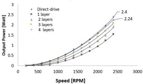
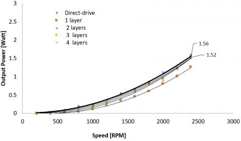
Figure 4 shows the test apparatus of the magnetic gear (n1 < n2). In the figure, both the magnetic gear is connected to the DC motor (n1) and DC generator (n2). The test system is able to measure the performance characteristics both accelerating and decelerating the magnetic gear. Measurements were taken in the loaded condition at variable speed, variable load, and the magnetic layer was varied, respectively. The measured data such as load current, output voltage, speed, and output power. The results of the comparison test of direct-drive with magnetic gear at speeds from 0-2400 rpm with a load of 200, 300, and 400 ohms are shown in Figures 5, 6, and 7, respectively.
Table 5. Variance and standard deviation of the magnetic layer flux of the primary magnetic gear
|
Magnet No. |
1 layer |
2 layers |
3 layers |
4 layers |
||||
|
$\overline{\mathbf{X}}_{1}$ |
$\overline{\mathbf{X}}_{1}^{2}$ |
$\overline{\mathbf{X}}_{2}$ |
$\overline{\mathbf{X}}_{2}^{2}$ |
$\overline{\mathbf{X}}_{3}$ |
$\overline{\mathbf{X}}_{3}^{2}$ |
$\overline{\mathbf{X}}_{4}$ |
$\overline{\mathbf{X}}_{4}^{2}$ |
|
|
1 |
87.7 |
7,685.4 |
173.3 |
30,044.4 |
235.0 |
55,225.0 |
278.3 |
77,469.4 |
|
2 |
98.7 |
9,735.1 |
194.7 |
37,895.1 |
239.7 |
57,440.1 |
272.3 |
74,165.4 |
|
3 |
78.3 |
6,136.1 |
177.0 |
31,329.0 |
217.3 |
47,233.8 |
257.3 |
66,220.4 |
|
4 |
75.3 |
5,675.1 |
161.7 |
26,136.1 |
216.3 |
46,800.1 |
269.7 |
72,720.1 |
|
5 |
85.3 |
7,281.8 |
167.7 |
28,112.1 |
230.7 |
53,207.1 |
255.7 |
65,365.4 |
|
6 |
76.0 |
5,776.0 |
168.7 |
28,448.4 |
223.0 |
49,729.0 |
244.7 |
59,861.8 |
|
7 |
85.0 |
7,225.0 |
166.7 |
27,777.8 |
206.0 |
42,436.0 |
259.7 |
67,426.8 |
|
8 |
90.0 |
8,100.0 |
174.0 |
30,276.0 |
221.0 |
48,841.0 |
253.3 |
64,177.8 |
|
9 |
79.3 |
6,293.8 |
172.0 |
29,584.0 |
233.0 |
54,289.0 |
262.7 |
68,993.8 |
|
10 |
84.3 |
7,112.1 |
223.7 |
50,026.8 |
258.0 |
66,564.0 |
274.0 |
75,076.0 |
|
11 |
82.0 |
6,724.0 |
178.0 |
31,684.0 |
228.0 |
51,984.0 |
258.0 |
66,564.0 |
|
12 |
82.7 |
6,833.8 |
168.3 |
28,336.1 |
220.7 |
48,693.8 |
252.3 |
63,672.1 |
|
13 |
82.0 |
6,724.0 |
166.3 |
27,666.8 |
231.3 |
53,515.1 |
253.3 |
64,177.8 |
|
14 |
87.7 |
7,685.4 |
178.7 |
31,921.8 |
219.3 |
48,107.1 |
217.7 |
47,378.8 |
|
15 |
93.7 |
8,773.4 |
171.7 |
29,469.4 |
211.3 |
44,661.8 |
233.0 |
54,289.0 |
|
16 |
86.3 |
7,453.4 |
174.7 |
30,508.4 |
214.7 |
46,081.8 |
225.7 |
50,925.4 |
|
Ʃ |
1354.3 |
11,5214.6 |
2,817 |
499,216.3 |
3,605.3 |
814,808.7 |
4067.7 |
103,8484.1 |
|
$\bar{X}$ |
84.7 |
176.6 |
225.3 |
254.3 |
||||
|
ƩXi2 |
1,834,218.8 |
7935489.0 |
12998428.4 |
12,998,428.4 |
||||
|
Variant (s2) |
38.4 |
216.6 |
160.6 |
160.5 |
||||
|
Standard deviation (s): 6.2 |
14.7 |
12.7 |
12.7 |
|||||
|
Standard error (se): 1.6 |
3.7 |
3.2 |
3.2 |
|||||
Table 6. Variance and standard deviation of the magnetic layer flux of the secondary magnetic gear
|
Magnet No. |
1 layer |
2 layers |
3 layers |
4 layers |
||||
|
$\overline{\mathbf{X}}_{1}$ |
$\overline{\mathbf{X}}_{1}^{2}$ |
$\overline{\mathbf{X}}_{2}$ |
$\overline{\mathbf{X}}_{2}^{2}$ |
$\overline{\mathbf{X}}_{3}$ |
$\overline{\mathbf{X}}_{3}^{2}$ |
$\overline{\mathbf{X}}_{4}$ |
$\overline{\mathbf{X}}_{4}^{2}$ |
|
|
1 |
85.0 |
7225.0 |
173.7 |
30160.1 |
225.7 |
50925.4 |
274.7 |
75441.8 |
|
2 |
81.3 |
6615.1 |
172.0 |
29584.0 |
223.7 |
50026.8 |
275.7 |
75992.1 |
|
3 |
79.7 |
6346.8 |
176.3 |
31093.4 |
246.0 |
60516.0 |
293.3 |
86044.4 |
|
4 |
82.3 |
6778.8 |
167.3 |
28000.4 |
236.7 |
56011.1 |
284.7 |
81035.1 |
|
5 |
84.7 |
7168.4 |
159.7 |
25493.4 |
210.0 |
44100.0 |
253.0 |
64009.0 |
|
6 |
86.7 |
7511.1 |
175.3 |
30741.8 |
240.3 |
57760.1 |
278.0 |
77284.0 |
|
7 |
94.3 |
8898.8 |
187.0 |
34969.0 |
225.7 |
50925.4 |
254.3 |
64685.4 |
|
8 |
88.7 |
7861.8 |
175.0 |
30625.0 |
229.0 |
52441.0 |
258.7 |
66908.4 |
|
Ʃ |
682.7 |
58405.8 |
1386.3 |
240667.2 |
1837.0 |
422705.9 |
2172.3 |
591400.3 |
|
$\bar{X}$ |
85.3 |
173.3 |
229.6 |
271.5 |
||||
|
ƩXi2 |
466033.8 |
1921920.1 |
3374569.0 |
4719032.1 |
||||
|
Variant (s2) |
21.7 |
61.3 |
126.4 |
217.3 |
||||
|
Standard deviation (s): 4.7 |
7.8 |
11.2 |
14.7 |
|||||
|
Standard error (se): 1.6 |
2.8 |
3.9 |
5.2 |
|||||
From Figures 5, 6, and 7, it can be seen that the addition of four magnetic layers in the magnetic gear can improve the magnetic force, therefore, we choose to arrange a piece magnet in parallel to meet assembly in gear's design. In other words, the addition of any one piece of the magnetic layer to the magnetic flux of 85.33 mT can improve magnetic-gear torque. Table 7 shows the increase in output power to the influence of the magnetic flux between the 4 magnetic layers and the direct drive with loads of 200, 300, and 400 ohms, respectively.
Figure 4. Axial MG prototype placed on the test bench (g=0.5mm)
Figure 5. The comparison between direct-drive and magnetic gear at load of 200 Ohm
Figure 6. The comparison between direct-drive and magnetic gear at load of 300 Ohm
Figure 7. The comparison between direct-drive and magnetic gear at load of 400 Ohm
Table 7. A comparison of the output power produced between a 4-layer magnetic gear with a direct drive with varying loads
|
No |
Loads (ohm) |
Output Power (Watts) |
|
|
Direct Drive |
Magnetic gear (4 layers) |
||
|
1. |
200 |
2.24 |
2.4 |
|
2. |
300 |
1.56 |
1.52 |
|
3. |
400 |
1.2 |
1.1 |
To compare the torque with varying loads with respect to each additional magnetic layer, the magnetic torque of the gear as a function of the number of magnetic layers with varying loads is shown in Figure 8. It is clear that the torque of magnetic gear will decrease in proportion to the output load at speed 2400 rpm. The figure indicates that the maximum load torque is applied to the direct coupling between the motor and the generator with a 200 Ohm loading of 0.19 x 10⁻³ (N-m).
Maximum load torque that occurs decreases proportional to the addition of load on the DC generator. Axial magnetic gear as proposed in Figure 1, each rectangular magnetic layer with 85.33 mT is capable of carrying a maximum load torque of 0.12 x 10⁻³ (N-m). The period of adding each layer to the rectangular magnet of the magnetic gear affects the increase in load torque. That is, the presence of four magnetic layers with the same magnetic flux strength approaches the maximum torque produced by the direct drive of 0.18 x 10⁻³ (Nm). In this test, the torque load ratio is only measured at the maximum load for direct drive. The aim is the basis of investigating the ability of each rectangular magnetic layer used in magnetic gear assembly.
Figure 8. Characteristics of load torque vs magnetic flux
3.3 Basic analogy of magnetic circuits vs electric circuits
Based on the theory of magnetism, there is a similar analogy to the electrical circuit. Therefore, to analyze the magnetic flux can be done with an electric circuit approach, known as Ohm's law:
$I=\frac{V}{R}$ (11)
where,
Thus, the replacement value of the above equation is:
$\Phi=\frac{\mathcal{F}}{\Re} \quad \leftrightarrow \quad I=\frac{V}{R}$ (12)
where,
From Eqns. (11) and (12), it can be described in terms of the circuit as shown in Figure 9.
Figure 9. Magnet circuit and electrical circuits: (a) Equivalent magnetic circuit and (b) Electrical circuit analogy
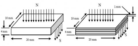
As an illustration, Figure 10 shows a comparison of the measurements of 1 magnetic bar with a thickness of 3 mm and 3 pieces of the magnet in parallel with a thickness of 1 mm. In this study, the result of magnetic flux measurements of magnetic layers in parallel with a thickness of 1 mm is 223 mT slightly higher than a magnet with a thickness of 3 mm, i.e. 196 mT. In addition, Figure 11 shows a magnet with a thickness of 4 mm versus 4 magnetic layers with a thickness of 1 mm. Here, the magnetic pole is illustrated that 1 rectangular magnet bar only has 2 poles, whereas a four-layer magnet has 8 poles.
Figure 10. Magnetic size 3 mm versus magnetic size 1 mm with 3 layers
Figure 11. An overview of the comparison of an NdFeB magnet pieces: (a) One layer of NdFeB magnets, (b) 4 layer of NdFeB magnets
3.4 Discussion
According to the paper [28], when rectangular magnetic tooth layers are arranged in parallel compared to in series, the magnetic reluctance decreases and increases magnetic flux. On the other hand, the presence of magnetic rectangular arranged in layers also leads to an increase in the number of poles. The torque of a magnetic gear depends on the number of magnetic poles, the area of the poles covered by the magnets, the magnetic field strength of magnets, and the separation distance between magnets of the coupling [19, 21].
For different multi-pole of the magnetic gears with the same magnetic field strength, the torque of magnetic coupling increases as the number of magnetic poles increases for distances smaller than the critical separation distance. This means that the magnetic force increases in proportion to the addition of four magnets arranged in parallel or it equals to add to 8 poles pairs. In this case, there are differences in the magnetic torque between four rectangular magnets arranged in parallel (multi-pole) with a thickness of 4 mm compared with a rectangular magnetic (2 poles) with the same thickness (Figure 11).
Table 8. Comparison of torque of several magnetic gear topologies
|
Topology |
Ratio |
Magnet Shape |
Remanence (T) |
Torgue (N-m) |
Ref. |
|
Planetary |
- |
sectoral |
1.09 |
24.13 |
[31] |
|
Coaxial |
1:5.5 |
coaxial |
1.25 |
24.5 |
[32] |
|
Spur (Radial) |
1:4 |
sectoral |
1.183 |
16.3 (analytic) 13.1 (measured) |
[24] |
|
Radial |
1:1 |
Rectangular |
1.16 |
5.29 |
[27] |
|
Radial |
1:16 |
sectoral |
1.3 |
2.6 |
[8] |
|
Parallel |
1:1 |
sectoral |
1.16 |
6.43 |
[33] |
|
Axial |
1:1 |
sectoral |
1 |
3.9 |
[33] |
|
Axial (serial) |
1:2 |
Rectangular |
0.099 |
1.9.10-3 (measured) |
[28] |
|
Axial (layers) |
1:2 |
Rectangular |
0.254 |
2.24.10-3 (measured) |
in this work |
On the other hand, Wu et al. [26] described an analytical approach for the transmitted torque calculation of an external magnetic gear set with rectangular magnets by employing the technique of the current sheet model. Based on the analytical model, the effects of design parameters, including the number of magnetic poles, the length of the air gap and the remanence of permanent magnets, affect the transmitted torque of magnetic gear.
Furthermore, the rectangular magnet composition of the layered system proposed in this paper is an attractive offer in the design of magnetic gear with several advantages. Among them, easy to make, very simple, it can provide increased torque compared to previous designs. Table 8 provides a comparison with some axial magnetic designs that have been made by previous researchers.
In this study, we developed axial magnetic gear using rectangular magnets with the most important conclusions obtained summarized as follows:
The authors would like to acknowledge the support of the Laboratory of Electrical Engineering, University of Nusa Cendana - Kupang and scholarship support from the Ministry of Research Technology and Higher Education.
|
I N |
current, Ampere north-pole |
|
NdFeB Nd2Fe l4B N-m Pm Rpm R S SmCo s se T V |
neodymium-iron-boron plastic bonded magnet newton-meter mechanical power repulsion per-meter resistance, Ohm south-pole samarium-cobalt standard deviation standard error torque, N-m voltage, Volt |
Greek symbol
|
Ф ω ℱ ℜ |
flux angular frequency of rotation, $2 \pi f n / 60$ magnetic force reluctance |
[1] Li, X., Chau, K.T., Cheng, M., Hua, W. (2013). Comparison of magnetic-geared permanent-magnet machines. Progress in Electromagnetics Research, 133: 177-198. https://doi.org/10.2528/PIER12080808
[2] Fu, W.N., Li, L.N. (2016). Optimal design of magnetic gears with a general pattern of permanent magnet arrangement. IEEE Transactions on Applied Superconductivity, 26(7). https://doi.org/10.1109/TASC.2016.2587279
[3] Gouda, E., Mezani, S., Baghli, L., Rezzoug, A. (2011). Comparative study between mechanical and magnetic planetary gears. IEEE Transactions on Magnetics, 47(2): 439-450. https://doi.org/10.1109/TMAG.2010.2090890
[4] Jian, L., Chau, K.T., Li, W., Li, J. (2010). A novel coaxial magnetic gear using bulk HTS for industrial applications. IEEE Trans. Appl. Supercond, 20(3): 981-984. https://doi.org/10.1109/TASC.2010.2040609
[5] Li, W., Chau, K.T., Li, J. (2011). Simulation of a tubular linear magnetic gear using HTS bulks for field modulation. IEEE Trans. Appl. Supercond, 21(3): 1167-1170. https://doi.org/10.1109/TASC.2010.2080255
[6] Liu, X., Chau, K.T., Jiang, J.Z., Yu, C. (2009). Design and analysis of interior-magnet outer-rotor concentric magnetic gears. J. Appl. Phys., 105(7): 97-101. https://doi.org/ 10.1063/1.3058619
[7] Atallah, K., Stuart, D., Calverley, Howe, D. (2004). High-performance magnetic gears. Journal of Magnetism and Magnetic Materials, 272-276: e1727-e1729. https://doi.org/10.1016/j.jmmm.2003.12.520
[8] Wu, Y.C., Jian, B.S. (2015). Magnetic field analysis of a coaxial magnetic gear mechanism by two-dimensional equivalent magnetic circuit network method and finite-element method. Applied Mathematical Modelling, 39: 5746-5758. https://doi.org/10.1016/j.apm.2014.11.058
[9] Husain, M. (2013). Design and development of magnetic variable transmission. Doctoral Dissertation, Osaka University Knowledge Archive: OUKA.
[10] Tsurumoto, K., Kikuchi, S. (1987). A new magnetic gear using permanent magnet. IEEE Transactions on Magnetics, 23(5): 3622-3624. https://doi.org/10.1109/TMAG.1987.1065208
[11] Kikuchi, S., Tsurumoto, K. (1993). Design and characteristics of magnetic worm gear using permanent magnet. IEEE Trans. Magn., 29: 2923-2925. https://doi.org/10.1109/20.280916
[12] Kikuchi, S., Tsurumoto, K. (1994). Trial construction of a new magnetic skew gear using permanent magnet. IEEE Trans., Magn., 30(6): 4767-4769. https://doi.org/10.1109/20.334216
[13] Ikuta, K., Makita, S., Arimoto, S. (1991). Non-contact magnetic gear for micro transmission mechanism. Proc. IEEE Conf. on Micro Electro Mechanical Systems. Nara, Japan, pp. 125-130. https://doi.org/10.1109/MEMSYS.1991.114782
[14] Atallah, K., Howe, D. (2001). A novel high-performance magnetic gear. IEEE Transactions on Magnetics, 37(4). https://doi.org/10.1109/20.951324
[15] Tsamakis, D.M., Ioannides, M.G., Nicolaides, G.K. (1996). Torque transfer through plastic bonded Nd2Fe14B magnetic gear system. Journal of Alloys and Compounds, 241: 175-179. https://doi.org/10.1016/0925-8388(96)02353-5
[16] Kramer, M.J., Mccallum, R.W., Anderson, I.A., Constantinides, S. (2012). Prospects for non-rare earth permanent magnets for traction motors and generators. Journal of the Minerals, Metals and Materials Society, 64(7): 752-763. https://doi.org/10.1007/s11837-012-0351-z
[17] Chen, M., Chau, K.T., Li, W., Liu, C. (2012). Development of non-rare-earth magnetic gears for electric vehicles. Journal of Asian Electric Vehicles, 10(2): 1607-1613. https://doi.org/10.4130/jaev.10.1607
[18] Wang, R., Furlani, P., Cendes, Z.J. (1994). Design and analysis of a permanent magnet axial coupling using 3D finite element field computations. IEEE Transactions on Magnetics, 30(4): 2292-2295. https://doi.org/10.1109/20.305733
[19] Mezani, S., Atallah, K., Howe, D. (2006). A high-performance axial-field magnetic gear. Journal of Applied Physics, 99: 08R303-1-3. https://doi.org/10.1063/1.2158966
[20] Yao, Y.D., Chiou, G.J., Huang, D.R., Wang, S.J. (1995). Theoretical computations for the torque of magnetic coupling. IEEE Transactions on Magnetics, 31(3): 1881-1884. https://doi.org/10.1109/20.376405
[21] Yao, Y.D., Huang, D.R., Hsieh, C.C., Chiang, D.Y., Wang, S.J., Ying, T.F. (1996). The radial magnetic coupling studies of perpendicular magnetic gears. IEEE Transactions on Magnetics, 32(5): 5061-5063. https://doi.org/10.1109/20.539490
[22] Yao, Y.D., Huang, D.R., Lee, C.M., Wang, S.J., Chiang, D.Y., Ying, T.F. (1997). Magnetic coupling studies between radial magnetic gears. IEEE Transactions on Magnetics, 33(5): 4236-4238. https://doi.org/10.1109/20.489760
[23] Yao, Y.D., Huang, D.R., Hsieh, C.C., Chiang, D.Y., Wang, S.J. (1997). Simulation study of the magnetic coupling between radial magnetic gears. IEEE Transactions on Magnetics, 33(2): 2203-2206. https://doi.org/10.1109/20.582770
[24] Jorgensen, F.T., Andersen, T.O., Rasmussen, P.O. (2005). Two dimensional model of a permanent magnet spur gear. Industry Applications Conference, pp. 261-265. https://doi.org/10.1109/IAS.2005.1518319
[25] Huang, C.C., Tsai, M.C., Dorrell, D.G., Lin, B.J. (2008). Development of a magnetic planetary gearbox. IEEE Transactions on Magnetics, 44(3): 403-412. https://doi.org/10.1109/TMAG.2007.914665
[26] Wu, Y.C., Wang, C.W. (2015). Transmitted torque analysis of a magnetic gear mechanism with rectangular magnets. Applied Mathematics & Information Sciences, pp. 1059-1065. https://doi.org/10.12785/amis/090257
[27] Wu, Y.C., Tseng, W.T., Chen, Y.C. (2013). Torque ripple suppression in an external-meshed magnetic gear train. Advances in Mechanical Engineering. https://doi.org/10.1155/2013/17899
[28] Syam, S., Soeparman S., Widhiyanuriyawan, D., Wahyudi, S. (2018). Comparison of axial magnetic gears based on magnetic composition topology differences. Energies, 11(153): 1-15. https://doi.org/10.3390/en11051153
[29] Huang, J., Wang, D., Zhang, D. (2012). The torque characteristic analysis and simulation on electromagnetic gears. Energy Procedia, published by Elsevier Ltd., pp. 1274-1280. https://doi.org/10.1016/j.egypro.2012.02.238
[30] Yao, Y.D., Chao, G.J., Huang, D.R., Wang, S.J. (1995). Theoretical computations for the torque of magnetic coupling. IEEE Transactions on Magnetics, 31(3). https://doi.org/10.1109/20.376405
[31] Kong, F.C., Zhu, X.Y., Quan, L., Ge, Y.M., Qiao, L. (2013). Optimizing design of magnetic planetary gearbox for reduction of cogging torque. IEEE Vehicle Power and Propulsion Conference (VPPC). https://doi.org/10.1109/VPPC.2013.6671697
[32] Jian, L., Chau, K.T., Gong, Y., Jiang, J.Z., Yu, C., Li, W. (2009). Comparison of coaxial magnetic gear with different topologies. IEEE Trans. Magn., 45: 4525-4529. https://10.1109/TMAG.2009.2021662
[33] Charpentier, J.F., Lemarquand, G. (2001). Mechanical behavior of axially magnetized permanent-magnet gears. IEEE Transactions on Magnetics, 37(3). https://doi.org/10.1109/20.920485