Mouad Garziad* | Abdelmjid Saka
OPEN ACCESS
The aim of this study is to examine the co-simulation strategies of dynamic modeling of powered two wheelers vehicle that will incorporate a wide engineering area. The model was developed by including multibody and dynamic modeling, control theory, and simulation considering several points in regards of design and physical characteristic. The article represents the outcome that contains the advantages of the co-simulation approach which is an important tool for modeling and dynamic analysis of a high complex system. Besides, the study goes further in explaining the methods of modelling the Powered Two Wheelers Vehicle containing various subsystems, and in several physical domains, where occur different energies: Mechanical, Electrical, Pneumatic, hydraulic, and Thermal, that dynamically interact. The results of this study may serve in identifying the influence of the rider behavior and his motion on the stability of the motorcycle. This study may contribute in improving the safety and stability in a critical situation of driving the vehicles, and the influence of biomechanical factors on dynamics driving.
motorcycle, modeling, MF tire, suspension, biomechanics, rider, stability, control
With the growing complexity of systems and technology in automotive fields, the Co-simulation become a more and more challenging task, therefore, in many engineering organizations, the design of the complete systems often demands tools that are used for testing and validating, as it needs a collaboration of different fields and from multiple domain of expertise. In Co-simulation, different subsystems, that coupled problems, are modeled and simulated in a divided way [1]. Consequently, and during simulation, the subsystems will exchange data and flow and effort flow. Co-simulation is indispensable and comprehensive view because it integrates many sub-systems. This approach is considered, therefore, as a joint simulation of tools and semantics already well established; when they are simulated with their appropriate solvers. Co-simulation demonstrate its capability to test and in the validation of multi domain and multi-physical systems by offering an effective solution that enables taking into consideration multiple domains with different time steps, at once. Since the Co-simulation give a positive result by enabling us to evaluate the system on a large and complex scale, generally, the Co-simulation use two or many different software that are integrated to ensure complete exchange of information.
Several studies were conducted based on Co-simulation in the field of vehicle engineering. Articles [2-7] portray the most significant sides and characteristics of the advanced multibody modeling of a motorcycle and virtual rider.
G. Sequenzia et al. [8] developed an approach based on Co-simulation for multibody parametric modeling of the motorcycle with an anthropomorphic model of the driver. Another substantial research was conducted by A. Khadr et al., [9] deals with modeling, simulation, design, and optimization of a semi-active suspension system using a fully dynamic model of a two-wheeled vehicle by using an optimization procedure, based on Genetic Algorithms.
This article represents a new approach based on Co-simulation in order to integrate all physical domain of the motorcycle considerate all different characteristic and aspects of the Powered Two Wheeled vehicle, that deal with stability, and path following. The first section will illustrate the configuration and physical characteristics of motorcycle and the necessary step for modelling the system. Moreover, the second section will provide the structuration and the different layers of a Co-simulation framework of motorcycle. Then, the third section will tackle the analysis of the performance and discussion of the main results and findings.
The general configuration depends on the physical functions, characteristics and the overall configuration of the motorcycle, for example, the kind of suspension system, the DOF of the system, the interaction between road and tire. In the case of our model, the multi-body model will consist of 11 rigid bodies; these latter will be interconnected using a number of joints like a revolute, spherical and prismatic joint. The description of the physical characteristics of the model of the motorcycle is significant since it determines, the configuration of the motorcycle, the degree of freedom, the number of rigid bodies, the number and the nature of the connections between the different bodies. The physical configuration of the motorcycle model can be described by:
All the features are presented below and explaining why these functions should be figured in the model of the motorcycle.
2.1 Characteristics of the front and rear suspension
The suspension is one of the parts that are necessary to shape a vehicle since it directly impacts the performance of vehicles and comfort of the ride. This latter is affected by the aspect of the suspension which importantly decreases the vibrations, shocks and forces caused by the Irregularities of the road. The modeling and development of this component is challenging. However, by including the suspension in the PTW vehicle, and adding four degrees of freedom: pitching motion, yaw movement around the Z axis and linear movements of the front and rear suspension.
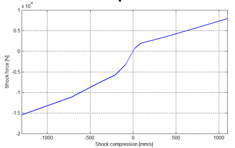
The total fork force is the end-stroke spring which represents the physical limit of the fork.
$F_{F f}=\left\{\begin{array}{ll} {-k_{\text {stop}}\left(s_{f}-s_{\text {min}, f}\right) \quad if s_{f}<s_{\text {min}, f} (bump stop)} \\ {0\quad if 0<s_{f}<s_{\min , f}} \\ {-k_{\text {stop}} s_{f} \quad if s_{f}>0 \quad (rebond stop)} \end{array}\right.$ (1)
where sf is df -lfrk is the stroke of the suspension, k is the stifness of the springs, $\Delta F_{f}$ is the preload and $\alpha$ represents the non linear stiffening of the spring, the total fork force is the end-stroke spring which represents the physical limit of the fork travel.
The damping force can be expressed by:
$F_{d}=\left\{\begin{array}{ll}{-c_{c} \dot{s}_{f}} & {\dot{s}_{f}<0} \\ {-c_{e} \dot{s}_{f}} & {\dot{s}_{f}>0}\end{array}\right.$ (2)
where Cc and Ce represent the damping expression in rebond and compression coefficient respectively, the force due to the helicoidal springs:
$F_{h s}=\Delta F_{f}-k\left(1+\alpha s_{f}\right) s_{f}$ (3)
The torque applied to the rear suspension is:
$M_{s w g}=\frac{\partial g}{\partial \gamma} F_{s h o k}=\eta F_{s h o k}$ (4)
where Fshok represents the shock force.
(a) Spring force vs spring compression
(b) Shock force vs shock compression
Figure 1. Suspension force charachterstic
2.2 Characteristic of tires
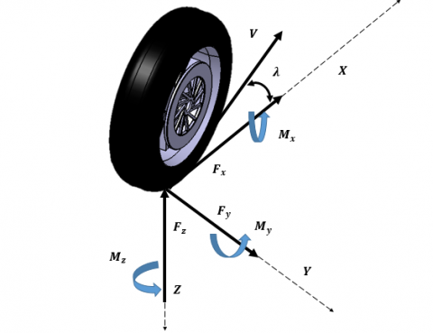
The tire is the most important components in the vehicle, so the performance of vehicles and comfort of the ride are largely influenced by the characteristics of the tires, the tire forces moments, longitudinal slip and sideslip are essential parameters for improving vehicle safety, steering ability and comfort. The orientation of force and moment of the tire are defined in the Figure 2.
Figure 2. Tire kinematic
There are two approach for modeling the tire; linear and nonlinear modelling, in the linear modelling, the tires are modeled as linear dampers and springs.
$\begin{aligned} F_{y f} &=C_{f 1} \alpha_{f}+C_{f 2} \varphi_{f} \\ F_{y r} &=C_{r 1} \alpha_{\mathrm{r}}+C_{r 2} \varphi_{r} \end{aligned}$ (5)
The nonlinear model is based on the Magic Formula, H. Pacejka [10] presents a recent model of the Magic Formula. The MF tire is sufficiently applicable to evaluate the general behavior of the vehicle but less applicable to evaluate the dynamic behavior of the tire in range of frequency limited to 8 Hz. Successful validation of the model of the motorcycle is entirely dependent on the contact described between the road and the vehicle due to the considerable influence of the properties of the tires on the driving of the vehicle. As a result, a tire model will be developed based on Pacejka's "magic formula". The model generates the longitudinal and lateral forces, and the aligning torque, in the form:
y(x)=Dsin$[\operatorname{Carctan}[(1-E) x+(E / B) \arctan (B X)]]$ (6)
where y(x) is the output variable and is defined as the longitudinal force $F_{x}=\mathrm{y}\left(\boldsymbol{k}, \boldsymbol{\alpha}, \boldsymbol{\gamma}, \boldsymbol{F}_{z}\right)$ or the lateral force, $F_{y}=\left(k, \alpha, \gamma, F_{z}\right)$, and self-aligning torque $\boldsymbol{M}_{\mathbf{z}}=\boldsymbol{M}_{\mathbf{z}}\left(\boldsymbol{k}, \boldsymbol{\alpha}, \boldsymbol{\gamma}, \boldsymbol{F}_{\mathbf{z}}\right)$, X is defined as the input variable: the longitudinal slip k as input for longitudinal forces or the lateral slip $\alpha$ as input for lateral forces. The interpretations of the remaining parameters in Equation are given in the LMS Virtual Lab software, the tire model is defined by a series of formulas that relate to the theory of the magic formula. For nonlinear simulation, a code is developed whose integrators include and DAE/ODE based algorithms, nonlinear motion differential equations being used, the only solution to predict kinematic and dynamic behavior is a digital time history of locations, orientations, forces, etc., each historical solution depends on the initial conditions chosen, and the result can sometimes vary considerably and unpredictably, even with small modifications of these initial conditions.
The following steps represent the overall architecture of the simulation program and the integration for the unit test and for the integration test necessary for the simulation of the dynamic behavior of the pneumatic element:
Figure 3. Architecture of the simulation of Tire
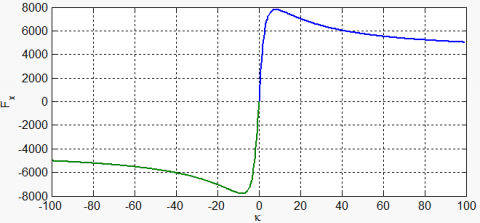
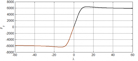
In the following plots, the results of pure interaction coefficients identification are presented:
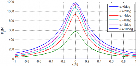
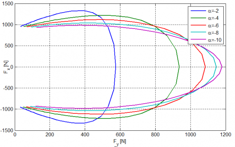
(a) longitudinal force (pure longitudinal slip)
(b) lateral force (pure side-slip)
(c) lateral force (pure longitudinal slip)
(d) longitudinal force (pure side-slip)
(e) lateral versus longitudinal force (combined slip)
Figure 4. Typical tire characteristics
The resulting diagrams describe some Typical Tire Characteristics, the figures show the variations of Fy and Fx been for several fixed values of side slip and pure slip, the lateral and longitudinal forces under pure and combined slip. The envelope of longitudinal and lateral tire forces, obtained by varying the side slip angle $\alpha$.
2.3 Biomechanical rider
In PTW vehicles, especially the bike, the rider accounts for nearly 90 % of mass and inertia. It is therefore important to directly quantify inertia, mass, and centers of mass. In order to understand the influence of rider, various rider and approaches for modeling the rider were used in the literature. Modeling a motorcycle rider is a difficult task. So the rider of automotive vehicle is limited in the output of the steering control to the interaction with the steering wheel, the rider of the motorcycle has a number of control options. The rider can use his handlebars to apply torque steering, move his weight by applying forces with his hands, feet, and knees [11-12].
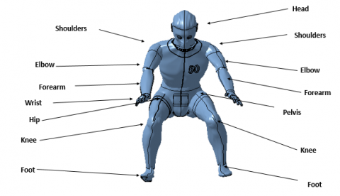
The LMS Virtual Lab modeling software was used to construct a parametric driver model, which could describe a modeling subject by developing a multibody model in a suitable form. Overall, the rider has 24 Degree of freedom, five of which are controlled, while the others are activated indirectly. The choice of the types of constraints applied to the connections between the different bodies was mainly based on the study of the kinematics activated by the rider while the execution of the maneuvers. The kind of joints composing the model are cited in Table 1:
Table 1. Mechanical joint and links
|
Connected bodies |
Joint type |
|
Arm-L - forearm-L |
Revolute joint |
|
Arm-R, forearm-R |
Revolute joint |
|
Forearm-L, front-frame, |
Revolute joint |
|
Forearm-R, front-frame, |
Revolute joint |
|
Arm-L, upper-body1 |
Spherical joint |
|
Arm-R, upper-body 1 |
Spherical joint |
|
Upper-body,lower-body |
Revolute joint |
|
lower-body, Upper Leg –L |
Revolute joint |
|
lower-body, Upper Leg –R |
Revolute joint |
|
Upper Leg-L, Lower Leg –L |
Spherical joint |
|
Upper Leg -R, Lower Leg –R |
Spherical joint |
|
Pelvis, main-frame |
Planar joint |
|
lower-body, main-frame |
Spherical joint |
|
Head – Neck |
Spherical joint |
|
Neck Upper-body |
Revolute joint |
|
Head- Torso |
Fixed joint |
Figure 5. Rider model
The constraints between the modeled driver and the motorcycle are:
Table 2 shows the characteristics stiffness of different parts of the rider body.
Table 2. Parameters of rider
|
Symbole |
Parameter |
Value |
|
Ky |
lateral displacement of the pelvis |
11935.63 Nm/rad |
|
cy |
Lateral displacement damping |
60.61 Nm/rad |
|
KH |
Arm stiffness |
257Nm |
|
CH |
Arm damping |
12.8 Nm |
|
K |
Roll stiffness (Pelvis - Torso) |
835 Nm/rad |
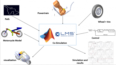
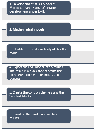
Co-simulation approach is a pertinent solution to beat this important challenge of modelling. It consists of the theory and techniques to enable global simulation of a given Multiphysics system. We present in an informal manner, the concepts that will be used throughout this modelling. The object if of this part is to connect the geometric model to the Simulink model. A control system has been created where the number of required inputs and outputs has been specified. The architecture diagram of the flow represented in Figure 6.
Figure 6. Architecture of co-simulation
The logic diagram shown in Figure 7 can realistically simulate the dynamics of the motorcycle rider system:
Figure 7. Architecture of the co-simulation technique
3.1 Multi-body modeling
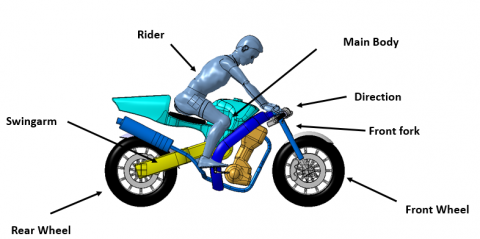
Figure 8. Motorcycle model
The dimensions of the components were chosen considering a real model of the motorcycle. The model consists 7 rigid bodies; the main body, the front fork, the front and rear suspension, the front and rear tires, and rider. These body parts are connected using appropriate joints in order to obtain the exact number of DOF. The considered PTW Vehicle contains a telescopic fork front suspension, a Swingarm rear suspension. The front includes the fork, handlebars, steering assembly, the front spring weight contains the lower fork and the front brake calipers. The road model is flat.
The rider has a prominent task in the control and the stability of motorcycle. Thus, the kinematics of the driver can be characterized and assessed according to the movement of the upper body, the trunk, the pelvis, the arms, and the legs. The driver's pelvis is particularly important because it is in direct contact with the chassis of the motorcycle. The geometric structure of the bodies and joints forming a rider is illustrated in Figure 8, it is assimilated to a poly-articulated arborescent structure of solids, and it is composed of 15 rigid bodies, the model of the driver comprises 15 rigid bodies. Our main task is to construct an integrated system of a rider and the motorcycle model which are interactive and dynamic. The action of the rider modifies the movements of the motorcycle, such as steering, leaning, and pitching of the body, weight shift, and knee grip, is represented by combining the D.O.F mentioned above as follows:
$T_{e l}=-K_{s t r_{P}}\left(\varphi_{d}-\varphi\right)-K_{s t r_{-} I} \int\left(\varphi_{d}-\varphi\right)+K_{s t r_{-} D} \dot{\varphi}$ (7)
where $\varphi_{d}$ is the desired lean angle.
$T_{\varphi}=-K_{L t r_{P}}\left(\varphi_{d}-\varphi\right)-K_{L t r_{-} I} \int\left(\varphi_{d}-\varphi\right)+K_{L t r_{-} D} \dot{\varphi}$ (8)
$T_{H}=K_{p 3}\left\{C_{2}\left(\varphi_{d}-\varphi_{r i d e r}\right)+\frac{1}{\tau_{i}} \int_{0}^{t} \tau_{i}\left(\varphi_{d}-\varphi_{r i d e r}\right) d t+\tau_{d}\left(\frac{d\left(\varphi_{d}-\varphi_{r i d e r}\right)}{d t}\right)\right\}$ (9)
where yd is the lateral displacement of the driver pelvis, and $\varphi_{\text {rider}}$, its angle of inclination of the torso.
$F=K_{p 2}\left\{C_{1}\left(\varphi_{d}-y_{d}\right)+\frac{1}{\tau_{i}} \int_{0}^{t} \tau_{p}\left(\varphi_{d}-y_{d}\right) d t+\tau_{d}\left(\frac{d y_{d}}{d t}\right)\right\}$ (10)
The remaining coefficients C1 and C2 are additional gains used to move the actuators from the active type to the passive type. Indeed, if C1 or C2 is zero, the corresponding expression returns the force (torque) generated by a linear (rotational) damping set.
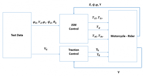
In this part, the control design has been described. First, the general control model is explained by giving a clear overview of the controller model structure. Secondly, the different kind of controllers are explained. This is done mainly by presenting the controller structure. The general control model is shown in Figure 9. The blocs represent Matlab functions, the error is calculated for both path tracking and stability criterion, for the stability of lean, yaw angle, and steering angle, velocity, and active action of rider.
Figure 9. Control structure
The analysis consisted of 3 successive steps: kinematic and dynamic modeling of the motorcycle rider system, Control, and simulation.
(a) Eigenvalues straight running motorcycle
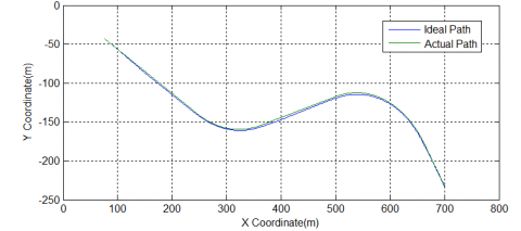
(b) Path following
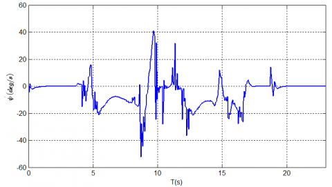
(c) Rider Lean angles
(d) Lean Rate angle
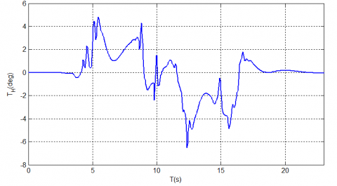
(e) Hip angle
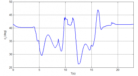
(f) Pitch angle of rider
(g) Steering torque
Figure 10. Simulation results
The results of the frequency analysis are presented in Figure 10.b, which shows the real part of the eigenvalues. The analysis is made in speed varies from 1 to 50 m/s. The vibratory modes in are highlighted are: weave, wobble. It can be seen that all modes tend to approach instability with increasing speed. This is natural if one thinks that with the increase of the speed, the energy available for the establishment of the movement also increases.
Although in this case, the wobble and weave modes remain well-damped over the entire speed range. The motorcycle does not exhibit stability problems at high speed under constant speed conditions. The damping in high-speed steer mode improves as the roll angle in steady-state increases, with increases being accompanied by increases in the frequency at high-speed steer mode. Increasing the roll angle has no marginal effect on high-speed sway damping, which is accompanied by a reduction in the sway frequency speed. The main criterion for a stabilized reversal mode is a vertical position of the motorcycle or an inclination of the vehicle corresponding to a lateral acceleration given by the radius of curvature.
The Figure 10.b shows the driven path by the controller compared with the path as described for the model. From the figure, it is concluded that the motorcycle model is driven correctly through the lane change. The rider model reacts in time and the slope of the path is steep enough to finish the maneuver in time. The model shows little overshoot, though it has a little too much undershoot. However, this is well within the limits of the lane change paths. The path control is based on the concept of the preview error and the actual error. The most important controller action is thought to be the feedforward preview control for the path.
The graphs show 10.g the steering torque that has a very good correlation with the lean rate with the yaw rate. The peak of especially the positive steering torque seems rather high, the maximum exerted a torque on the handlebars is 30 N.m for a time period of less than a second. It has been a very dynamical one which required a subjectively reasonable amount of effort.
The graphs show lean and yaw rates, the simulated lean rate, it has a qualitatively similar result compared with the steering angle, and the results look very promising.
To conclude, the co-simulation is an essential step of modeling and dynamic analysis; it which represents a unified approach and powerful tool for modeling a Multiphysics system, control, and diagnosis of Two-wheeled vehicles. Not only that but we can define the PTW as a mechatronic system, where run several energies: mechanical, electrical, pneumatic, thermal it is submissive to many problems, strong coupling with the environmental sub-systems and variant energies. In point of fact four levels of modeling (technological, physical, mathematical and algorithmic) can be presented due to its functional, structural, behavioral and causal properties. In addition, vehicles are complex systems consisting of different subsystems in many physical domains that dynamically interact. In this regard, co-simulation strategies are particularly attractive as each subsystem is solved via tailored simulation tools with appropriate numerical methods regarding efficiency, and accuracy and integrating all fields. In this article, we presented the co-simulation strategies of dynamic modeling of the motorcycle. The research covered a wide range of topics, including modeling, simulation, and control of two-wheeled vehicles respecting a number of design and analysis considerations, including the integration of dynamics. Not only that, but we dealt also with another potential interest which showed how the knowledge of human behavior on the dynamics of a road vehicle and test the impact of the driver's motion on the behavior of the motorcycle and ameliorate the safety and security in an existed environment.
It is recommended to develop and implement an intelligent tool that secures the driver. This tool would be useful in assessing the body movements in real time and automatically distinguish normal driving after an accident using advanced algorithms, as to recognize the relevant characteristics, driving parameters (driving style, road characteristics, handling of curves).
[1] Gomes, C., Thule, C., Broman, D., Larsen, P.G., Vangheluwe, H. (2017). Co-simulation: State of the art. arXiv preprint arXiv:1702.00686.
[2] de Almeida, Eng Pedro Miguel. Biomechanical Model, https://www.researchomatic.com/Biomechanical-Model-123635.html, accessed on Jan. 8, 2019.
[3] Cali, M., Oliveri, S.M., Sequenzia, G., Trovato, F. (2018). Geometric and multibody modeling of rider-motorcycle system. 20th European Modeling & Simulation Symposium, Campora S. Giovanni, Italy, 2008.
[4] Saccon, A., Hauser, J., Beghi, A. (2008). A virtual rider for motorcycles: An approach based on optimal control and maneuver regulation. 3rd International symposium on communications, control and signal processing (ISCCSP), Malta, 2008, pp. 243-248. https://doi.org/10.1109/ISCCSP.2008.4537227
[5] Cali, M., Oliveri, S.M., Sequenzia, G., Trovato, F. (2008). Geometric and multibody modeling of rider-motorcycle system. In: 20th European modeling & simulation symposium, Campora S. Giovanni, Italy, 2008.
[6] Keppler, V. (2010). Analysis of the biomechanical interaction between rider and motorcycle by means of an active rider model. Proceedings, Bicycle and Motorcycle Dynamics 2010 Symposium on the Dynamics and Control of Single Track Vehicles, 20–22 October 2010, Delft, The Netherlands.
[7] Barbagallo, R., Sequenzia, G., Oliveri, S.M., Cammarata, A. (2016). Dynamics of a high-performance motorcycle by an advanced multibody/control co-simulation. Proceedings of the Institution of Mechanical Engineers, Part K: Journal of Multi-body Dynamics, 230(2): 207-221. https://doi.org/10.1177/1464419315602825
[8] Sequenzia, G., Oliveri, S.M., Fatuzzo, G., Calì, M. (2015). An advanced multibody model for evaluating rider’s influence on motorcycle dynamics. Proceedings of the Institution of Mechanical Engineers, Part K: Journal of Multi-body Dynamics, 229(2): 193-207. https://doi.org/10.1177/1464419314557686
[9] Khadr, A., Houidi, A., Romdhane, L. (2013). Development of co-simulation environment with ADAMS/Simulink to study maneuvers of a scooter. Design and Modeling of Mechanical Systems. Springer, Berlin, Heidelberg, pp. 37-43. https://doi.org/10.1007/978-3-642-37143-1_5
[10] Pacejka, H. (2005). Tire and vehicle dynamics. New York: Elsevier.
[11] Imaizumi, Hi., Fujioka, T. (1995). Motorcycle dynamics by multibody dynamics analysis. SAE Technical Paper. https://doi.org/10.4271/951806
[12] Imaizumi, H., Fujioka, T., Omae, M. (1996). Rider model by use of multibody dynamics analysis. JSAE Review, 17(1): 75-77. https://doi.org/10.1016/0389-4304(95)00057-7