Manju Singh* | Vijay Khare
© 2022 IIETA. This article is published by IIETA and is licensed under the CC BY 4.0 license (http://creativecommons.org/licenses/by/4.0/).
OPEN ACCESS
This study intends to propose a PD detection using spiral sketching and CNN. The fundamental idea is to analyze a person's spiral drawings and classify them as healthy or having Parkinson's disease. Spiral sketches drawn by healthy people look almost like standard spiral shapes. However, the spirals drawn by people with Parkinson's disease look distorted because they deviate significantly from their perfect spiral shape due to slow movement, and poor hand-brain coordination. In this paper Convolution, Neural Network is used to detect Parkinson’s, and 83.6% classification accuracy is obtained.
spiral drawing, Parkinson’s disease convolution neural network
PD is indeed the second most frequent neurological condition in the elderly, after Alzheimer's. The exact etiology of Parkinson's disease is unknown; however, genes and environment have a role. Parkinson's disease symptoms are normally appeared gradually and progressively worsen. Patients may find it difficult to walk and speak as their sickness develops. Parkinson's disease affects both males and women. Men are around 50% more likely affected than women with this disease. Parkinson's disease has an evident risk factor: age. The majority of persons with Parkinson's disease acquire symptoms around the age of 60, however about 5-10% of those who show symptoms before the age of 50 have "early onset" disease. Parkinson's disease is hereditary in many cases, but not all. Some varieties are linked to specific genetic abnormalities [1-3]. Patients experience resting tremors, bradykinesia, and stiffness issues as a result of this. Fatigue, anxiety, depression, slowed thinking, and voice troubles are some of the additional symptoms.
Dopamine’s a sort of neurotransmitter generated by neurons that helps them convey signals to other neural connections. Degeneration among these dopamine neurons in the substantial nigra causes Parkinson's disease. Movement abnormalities are caused by neurons dying or becoming damaged, which produces less dopamine. Scientists are still unsure what causes dopamine-producing cells to die. Nerve endings that produce norepinephrine, a crucial chemical messenger of the sympathetically nervous system that controls numerous physical activities such as increased heart rate, are also lost in people with Parkinson's disease [4-5]. Fatigue, uneven blood pressure, slower food passage through the gastrointestinal, and a quick decrease in the level when a person sits or sticks up from a reclining position are all symptoms of norepinephrine loss in Parkinson's disease. It might assist in understanding some of the characteristics. Lewy bodies, an aberrant mass of the protein -synuclein, are found in many brain cells in persons with Parkinson's disease. Scientists are striving to figure out, how alpha-synuclein functions normally and abnormally, as well as the genetic abnormalities that cause PD and Lewy body neurological diseases. In some PD effected persons occurrences of Parkinson's disease appeared to be hereditary and, in few cases, PD can be linked to specific genetic changes, the disease is most often unintentional and not runs in families. Many experts now believe Parkinson's disease is caused by a combination of hereditary and environmental factors, such as toxic exposure. PD is a progressive neuro-degeneration that affects the human brain's motor system. Early dosing can give the patient immediate comfort while also slowing the progress of Parkinson's disease [6-8].
Impaired handwriting in PD patients may appear years before a clinical diagnosis is made and, thus, could be the first signs of possible PD. By assessing handwriting via a digitizer, which measures the mean pressure and means velocity, as well as the spatial and temporal characteristics of every stroke [9]. Correct PD detection is a difficult task. If a patient has PD but is mistakenly diagnosed as healthy, the illness can progress and become difficult to manage. Several medical tests can detect it. However, because it's far linked to organic alterations in the brain, detection by visible image evaluation is the best strategy. PET and SRECT are imaging techniques commonly used in the diagnosis of Parkinson's disease. Furthermore, few studies show that those imaging modalities may accurately diagnose Parkinson's disease. [10-11]. However, medical experts do not choose to adopt those strategies because of their sensitivity and high expense. Magnetic Resonance Imaging (MRI) is still a harmless screening tool that is rarely used to detect Parkinson's disease. However, recent advances in MRI have made identification more straightforward. Bayes, Decision Tree, Support Vector Machine (SVM), and Artificial Neural Network are some of the classifying algorithms that have been employed to detect PD in MRI images.
CNNs (Convolutional Neural Networks) are ubiquitous. This is the most often used deep learning architecture. Convolutional Neural Network (CNN) is a biologically stimulated Deep Neural Network (DNN) technique that does not require hand-made skills. CNN's self-characteristic mastery capability allows it to exceed many fresh results in computer vision problems [12-14]. The enormous popularity and efficacy of convnet have sparked a recent surge in curiosity in deep learning. CNN has become the go-to resource for image-related difficulties. They blow the competitors out of the water in terms of precision. It also applies to suggested systems, speech recognition, and other areas. The fundamental advantage of CNN over its counterpart is that it discovers essential traits without the need for human intervention. Many photographs of cats and dogs, for example, are used to teach students about the self-looking functions for every class. CNN is also efficient mathematically. Using specific search and pool procedures, perform a parameter release. CNN models may now run across any device, offering them globally appealing. Everything about the sounds seems to be a pure enchantment. A model that uses automatic feature extraction to reach superhuman precision. Hopefully, this information will assist us in unraveling the mystery surrounding this incredible technology [15].
Using Spiral Drawings as well as Convolutional Neural Networks, this research provides a solution for identifying Parkinson's disease (CNN)as shown in Figure 1. The Google collab platform is utilized for implementation since it allows for the seamless execution of python notebooks for building AI structures that can eventually be deployed on the border.
Figure 1. CNN – 4-layer architecture
2.1 Dataset
The Parkinson drawing collection was used in this study. Images of spirals and waves painted in healthy people and persons with Parkinson's disease are included in the dataset. Only spiral drawings are used to classify this item. With no need to actively separate the dataset because it already comprises a train set as well as a test set.
The researchers looked at 55 age-matched volunteers ranging from UPDRS = 0 (CG) to significantly disturbed patients (UPDRS> 24). All PD subjects were enrolled via Dandenong Neurology's PD Outpatient Department in Melbourne, Australia, while CG subjects were recruited through word-of-mouth and correctly placed posters from multiple aged care homes. All of the participants were dominantly right-handed. CG individuals were chosen to closely resemble the age and gender distribution of PD patients. Skeletal injuries, neuroma and musculoskeletal problems, and excess levodopa medicines that cause dyskinesias were also considered exclusion criteria. The investigation was carried out on Parkinson's disease patients who were taking levodopa. Table 1 shows demographic and clinical information.
Table 1. Participant’s demographic and clinical information
|
|
Control group |
Parkinson’s disease |
|
Demographics |
|
|
|
Number of subjects,n |
28 |
27 |
|
Age, years |
71.32±7.21 |
71.41±9.37 |
|
Gender male/female |
21/6 |
22/6 |
|
Clinical information |
|
|
|
Disease duration, years |
- |
6.7±4.44 |
|
Unified Parkinson’s Disease Rating Scale-III |
- |
17.59±7.69 |
Values are represented as mean±SD
A certified neurologist assessed the severity of myopathy in all patients using Section 3 (Q1831) of both the UPDRS score and the general PD staging was determined using the modified Hoehn & Yahr measure (H & Y). Has been executed. CG has no PD symptoms indicated by SL 0. Additional groups were categorized as SL: 1–3 based on the UPDRS III (20) and also the updated H and Y evaluations (21, 22). (See Table 2). There were no late-stage illnesses or bedridden patients.
Table 2. Groupings depend on severity
|
SL |
Numberof subjects |
Unified Parkinson’s Disease Rating Scale (UPDRS) Sec III score(0-56) |
UPDRS Means±SD |
Modified H&Y stages (Sec V) |
|
0 |
28 |
0 |
- |
0 |
|
1 |
12 |
˃0 and ˂15 |
10.75±2.18 |
1, 1.5 |
|
2 |
8 |
≥15 and ≤23 |
18.38±2.83 |
2, 2.5 |
|
3 |
7 |
˃24 |
28.43±2.64 |
≥3 |
2.2 Data distribution
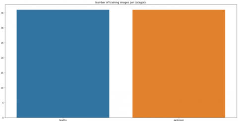
The following charts show the data spread of the Train and Test sets. When a data set is divided into such a training dataset and then a testing set, the 75% of the data should be used for training, and a 25% is utilized for testing.
Figure 2. No. of training images per category
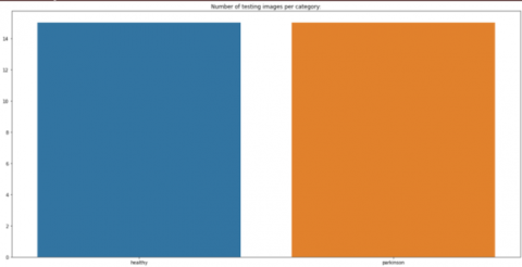
Figure 3. No. of testing images per category
The information is already balanced, as shown in Figure 2 and Figure 3. However, both the train and test sets of the dataset have much fewer photos per category. As a result, the next part shows how to extend the dataset to create artificial visuals for training and validation.
2.3 Data augmentation
In data analysis, data extension is a technique for adding a slightly tweaked replica of current data or freshly created synthetic data utilizing existing data to enhance the quantity of data available. When building machine learning models, it functions as a regularized and helps to reduce overfitting. This is directly related to data analysis oversampling. Machine learning applications are quickly diversifying and expanding, particularly in deep learning. Data augmentation technology has become an essential tool for addressing artificial intelligence's difficulties. By adding new examples to training datasets, data enrichment improves the performance and outputs of machine learning models. The model's effectiveness will be substantially better if the dataset is rich & sufficient. Collecting and categorizing data for machine learning techniques can be a time-consuming and costly procedure. Data augmentation technology will help enterprises decrease these operational costs by transforming datasets. Cleaning the data is one of the phases in the data model. For fidelity models, this is required. However, if cleaning diminishes the data's expressiveness, the model will be unable to produce good estimations for the respondents. By introducing variations that that model can observe in the actual world, data augmentation technologies have made machine learning models more resilient. The code below shows how to leverage the data expansion procedure to make an image and raise the dataset's size artificially. To create a new image, I am using the image data generator. Because the image is a spiral, it may be turned to any degree without losing its meaning. The rotational range is set at 360. You can experiment with the Image Data Generator class's other image conversions. However, be cautious when using extensions, as some changes can degrade the CNN model's accuracy. While training your model, Image Data Generator allows me to scale images in real-time. Any random transformation can be applied to the training image provided to the model. This not only strengthens the model but also saves memory.
2.4 Visualize images of trains and test sets
Here we visualize the images contained in the dataset.
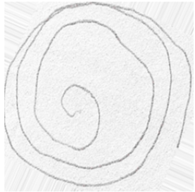
1) Images in train set: This is the output you get when you run the code to visualize the image. Figure 4 shows a spiral drawing image created by a healthy person, and Figure 5 shows a spiral drawing image created by a person with Parkinson's disease in a training dataset.
Figure 4. Spiral by a healthy person
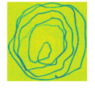
Figure 5. Spiral drawing by the individual who has Parkinson’s disease
2) Images in the test set: Figure 6 shows a spiral drawing image created by a healthy person, and Figure 7 shows a spiral drawing image created in the test dataset by a person suffering from Parkinson's disease.
Figure 6. Spiral drawing by a healthy person
Figure 7. Spiral drawing by a person having Parkinson’s disease
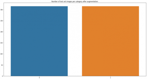
2.5 The data distribution after augmentation
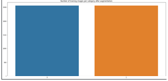
The following Figures 8 and 9 show the distribution of the dataset after the expansion process performed in the above area.
Figure 8. No. of images per category after augmentation
Figure 9. No. of the test set images after augmentation
2.6 Convolution neural network model
The implementation employs a CNN architecture that includes the following features:
The model has four convolution layers with filters of 128, 64, 32, and 32. Each convoluted layer is followed by a MaxPool 2D layer, which contains filters of varying filter sizes. Maximum pooling is a procedure that represents the Maximum score for each patch within every feature map. The convolution block is followed by two fully connected layers, which have been found to operate better than the typical pooling of machine learning applications such as image identification. With flattened inputs, a fully connected layer connects all neurons. The FC layer, if present, is usually found at the conclusion of the CNN design and can be utilized to optimize goals like class evaluation [16-22].
This part gives an overview of the entire model. This includes four convolution layers, each convolution layer has a maxpool2d layer and two completely connected layers.
Model: sequential 1
Layer [type] Output Shape Parameters
--------------------------------------------------------------------------
conv1 [Conv2D] (None, 128, 128, 128) 3328
--------------------------------------------------------------------------
max pooling2- 4 (MaxPooling2 (None, 40, 40, 128) zero
--------------------------------------------------------------------------
conv2 [Conv2D] (None, 40, 40, 64) 204864
max pooling2d-5 (MaxPooling2 (None, 12, 12, 64) zero
--------------------------------------------------------------------------
conv3 [Conv2D] (None, 12, 12, 32) 18464
--------------------------------------------------------------------------
Max pooling2d-6 (MaxPooling2 (None, 4, 4, 32) zero
------------------------------------------------------------------ -------
conv4 [Conv2D] (None, 4, 4, 32) 9248
--------------------------------------------------------------------------
Max pooling2d-7 (MaxPooling2 (None, 1, 1, 32) zero
--------------------------------------------------------------------------
Flatten-1 [Flatten] (None, 32) zero
--------------------------------------------------------------------------
Dropout-2 [Dropout] (None, 32) zero
--------------------------------------------------------------------------
fc1 [Dense] (None, 64) 2112
--------------------------------------------------------------------------
Dropout-3 [Dropout] (None, 64) zero
--------------------------------------------------------------------------
Fc2 [Dense] (None, 2) 130
--------------------------------------------------------------------------
238,146 parameters total
238,146 trainable parameters
Zero are non-trainable parameters.
The first input layer has no learnable parameter. Parameters in the second
CONV1(filter shape $=5 \times 5$, stride $=1)$
$ \text { layer } \text { is } =((\text { shape of width of filter } \times \text { shape of height filter } \times \text { stride }+1) \times \text { number of filters }) =(((5 \times 5 \times 1)+1) \times 128)=3,328$
The pooling layer has no parameters.
Parameters in the fourth CONV2(filter shape $=5 \times 5 \text {, stride }=1)$
layer is $=($ (shape of width of filter$\times$ shape of height filter$\times$ number of filters in previous layer
$+1) \times$ number of filters $)=(((5 \times 5 \times 128)+1) \times 64)$$=2,04,864$
Parameters in the CONV3 $=(((3 \times 3 \times 64)+1) \times 32)$ $=18,464$
Parameter in the CONV4 $=(((3 \times 3 \times 32)+1) \times 32)$ $=9,248$
Parameters in the FC1 layer is ((current layer $c \times$ $\times$ previous layer $p)+1 \times c)$ $=(32+1) \times 64=2112$
Parameter in the FC2 layer is: $((\text { current layer } c \times \text { previous layer } p) +1 \times c)=(64+1) \times 2=130$
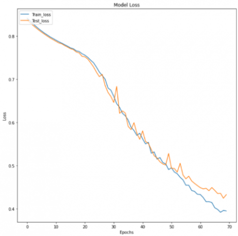
The Adam Optimizer is used to train the model, which has a linear function of 3.15e5. Adam is a new optimization technique that can replace the classic gradient-descent method of updating network weights learned from the training data. Adam is not the same as the traditional stochastic gradient descent approach. For all weight updates, stochastic gradient descent uses a single learning algorithm (called alpha), which does not fluctuate during training. Each network component (parameter) maintains its learning rate, which is modified independently as learning occurs. The size of both the epoch & stack is set to 70 (seventy) and 128 (one hundred and twenty eight), correspondingly.
Model performance is measured using loss and efficiency charts and classification reports. Figures 10 and 11 shows the accuracy of the model.
Figure 10. Model accuracy
Figure 11. Model loss
Below the analysis and results the model of two photos. The following diagram depicts the outcomes: Figure 12 shows a model prediction image of a healthy subject, and Figure 13 shows a model prediction image of a Parkinson's disease subject.
Figure 12. Model prediction as healthy person
Figure 13. Model prediction as person having disease
This is the classification report has been shown in form of Confusion matrix in Table 3.
Table 3. Confusion matrix for Parkinson’s disease analysis
|
Total=55 |
Predicate NO |
Predicate yes |
|
|
Actual No |
TN=21 |
FP=7 |
28 |
|
Actual yes |
FN=2 |
TP=25 |
27 |
|
|
23 |
32 |
|
Accuracy $=\frac{T P+T N}{T o t a l} \times 100=\frac{25+21}{55} \times 100=83.6 \%$ (1)
Error rate $=\frac{F P+F N}{\text { Total }}=\frac{7+2}{55} \times 100=16.3 \%$ (2)
True positive rate $($ recall $)=\frac{\text { TP }}{\text { Actual yes }} \times 100=\frac{25}{27} \times 100=92.5 \%$ (3)
also known as “Sensitivity”.
False positive Rate $=\frac{F P}{\text { actual no. }} \times 100=\frac{7}{28} \times 100=25 \%$ (4)
True negative Rate $($ Specificity $)=\frac{T N}{\text { actual no }} \times 100=\frac{21}{28} \times 100=75 \%$ (5)
Precision $=\frac{T P}{\text { Predicted yes }} \times 100=\frac{25}{32} \times 100=78.1 \%$ (6)
In this study, Detection of PD person using spiral sketching and CNN has been done. The idea is to analyze a person's spiral drawings and classify them as healthy or having Parkinson's disease. The goal of this study is to optimize the model so that it has fewer than 250,000 parameters and is simple to deploy to peripheral devices. This methodology gives a CNN-based Parkinson's disease identification solution that may be used on inefficient or edge devices. By using CNN classifier 83.6% classification accuracy is obtained.
In Parkinson's disease, the ability of sketching and writing of patience is decreased with severity, authors focus on this biomarker and developed a CNN-based model for understanding the pattern in sketching for the detection of PD. By using a convolutional neural network, we can classify the sketches made by Parkinson's patients and healthy subjects and obtain 83.6% accuracy, a sensitivity of 92.5%, a precision of 78.1%, specificity of 75%for both classes respectively. Now as the classifier report seems to be good, there is always the possibility to improve the methodology and performance of the classifier. The improvement can be made in the current methodology that the number of data samples can be increased significantly, and different types of drawing apart from the spiral and another CNN model must be employed. But the proposed model empowers us with much confidence that it can be used for the detection of Parkinson's disease in real life.
We declare that this manuscript is original, has not been published before, and is not currently being considered for publication elsewhere. We know no conflicts of interest associated with this publication, and there has been no significant financial support for this work that could have influenced its outcome. As Corresponding Author, I confirm that the manuscript has been read and approved for submission by all the named authors. We have used well known available standard data set. So ethical approval was not required for this study. Because we have not collected new data or perform any experiment for this study. All authors approved the final version of the manuscript and agree to be accountable for all aspects of this work.
[1] Goldenberg, M.M. (2008). Medical management of Parkinson’s disease. P&T, 33(10): 590-606.
[2] Parkinson's Disease Symptoms. Mayo Clinic. http://www.mayoclinic.org/diseasesconditions/parkinsons-disease/basics/symptoms/con-20028488, accessed on Sep. 13, 2017.
[3] Jankovic, J. (2008). Parkinson's disease: Clinical features and diagnosis. Journal of Neurology, Neurosurgery & Psychiatry, 79(4): 368-376. https://doi.org/10.1136/jnnp.2007.131045
[4] Prashanth, R., Roy, S.D., Mandal, P.K., Ghosh, S. (2014). Automatic classification and prediction models for early Parkinson’s disease diagnosis from SPECT imaging. Expert Systems with Applications, 41(7): 3333-3342. https://doi.org/10.1016/j.eswa.2013.11.031
[5] Pham, H.N., Do, T.T.T., Chan, K.Y.J., Sen, G., Han, A.Y.K., Lim, P., Loon Cheng, T.S., Nguyen, Q.H., Nguyen, B.P., Chua, M.C.H. (2019). Multimodal detection of Parkinson disease based on vocal and improved spiral test. In 2019 International Conference on System Science and Engineering (ICSSE), pp. 279-284. https://doi.org/10.1109/ICSSE.2019.8823309
[6] Luo, C.Y., Chen, Q., Song, W., Chen, K., Guo, X.Y., Yang, J., Huang, X.Q., Gong, Q.Y., Shang, H.F. (2013). Resting-state fMRI study on drug-naive patients with Parkinson's disease and with depression. Journal of Neurology, Neurosurgery & Psychiatry, 85(6): 675-683. http://dx.doi.org/10.1136/jnnp-2013-306237
[7] Parkinson's Progression Markers Initiative. http://www.ppmi-info.org/, accessed on accessed on Sep. 13, 2017.
[8] Rumman, M., Tasneem, A.N., Farzana, S., Pavel, M.I., Alam, M.A. (2018). Early detection of Parkinson’s disease using image processing and artificial neural network. In 2018 Joint 7th International Conference on Informatics, Electronics & Vision (ICIEV) and 2018 2nd International Conference on Imaging, Vision & Pattern Recognition (icIVPR), IEEE, pp. 256-261. https://doi.org/10.1109/ICIEV.2018.8641081
[9] Parisi, L., Ma, R.F., Zaernia, A., Youseffi, M. (2021). Ηyper-sinh-convolutional neural network for early detection of Parkinson’s disease from spiral drawings. WSEAS Trans Comput. Res, 9: 1-7. http://dx.doi.org/10.37394/232018.2021.9.1
[10] Marras, C., Beck, J.C., Bower, J.H., Roberts, E., Ritz, B., Ross, G.W., Abbott, R.D., Savica, R., Van Den Eeden, S.K., Willis, A.W., Tanner, C.M. (2018). Prevalence of Parkinson’s disease across North America. NPJ Parkinson’s Disease, 4: 21. https://doi.org/10.1038/s41531-018-0058-0
[11] Acharya, U.R., Oh, S.L., Hagiwar, Y., Tan, J.H., Adeli, H. (2018). Deep convolutional neural network for the automated detection and diagnosis of seizure using EEG signals. Comput Biol Med, 100: 270-278. https://doi.org/10.1016/j.compbiomed.2017.09.017
[12] Yu, L., Chen, H., Dou, Q., Qin, J., Heng, P.A. (2017). Automated melanoma recognition in dermoscopy images via very deep residual networks. IEEE Trans Med Imaging, 36(4): 994-1004. https://doi.org/10.1109/tmi.2016.2642839
[13] Liu, M., Zhang, J., Adeli, E., Shen, D. (2018). Landmark-based deep multi-instance learning for brain disease diagnosis. Med Image Anal., 43: 157-168. https://doi.org/10.1016/j.media.2017.10.005
[14] Shahid, A.H., Singh, M.P. (2019). Computational intelligence techniques for medical diagnosis and prognosis: Problems and current developments. Biocybern Biomed Eng., 39(3): 638-672. https://doi.org/10.1016/j.bbe.2019.05.010
[15] Krizhevsky, A., Sutskever, I., Hinton, G.E. (2017). Imagenet classification with deep convolutional neural networks. Advances in Neural Information Processing Systems. Red Hook: Curran Associates Inc., 60(6): 84-90. https://doi.org/10.1145/3065386
[16] Shi, J., Xue, Z.Y., Dai, Y.K., Peng, B., Dong, Y., Zhang, Q., Zhang, Y.C. (2019). Cascaded multi-column rvfl+ classifier for single-modal neuroimaging-based diagnosis of Parkinson’s disease. IEEE Transactions on Biomedical Engineering, 66(8): 2362-2371. https://doi.org/10.1109/TBME.2018.2889398
[17] Szegedy, C., Liu, W., Jia, Y.Q., Sermanet, P., Reed, S., Anguelov, D., Erhan, D., Vanhoucke, V., Rabinovich, A. (2015). Going deeper with convolutions. In: Proceedings of the IEEE Conference on Computer Vision and Pattern Recognition. https://doi.org/10.1109/CVPR.2015.7298594
[18] Xue, L.Y., Hou, Y., Wang, S.W., Luo, C., Xia, Z.Y., Qin, G., Liu, S., Wang, Z.L., Gao, W.S., Yang, K. (2022). A dual-selective channel attention network for osteoporosis prediction in computed tomography images of lumbar spine. Acadlore Trans. Mach. Learn., 1(1): 30-39. https://doi.org/10.56578/ataiml010105
[19] Rehman, A., Butt, M. A., Zaman, M. (2022). Liver lesion segmentation using deep learning models, Acadlore Trans. Mach. Learn., 1(1), 61-67. https://doi.org/10.56578/ataiml010108
[20] Kale, A.P., Sonawane, S., Wahul, R.M., Dudhedia, M.A. (2022). Improved genetic optimized feature selection for online sequential extreme learning machine. Ingénierie des Systèmes d’Information, 27(5): 843-848. https://doi.org/10.18280/isi.270519
[21] Jonnala, P., Reddy, U.J. (2019). Secured data representation in images using graph wavelet transformation technique. Ingénierie des Systèmes d’Information, 24(2): 177-181. https://doi.org/10.18280/isi.240208
[22] Mikolov, T., Deoras, A., Povey, D., Burget, L., Černocký, J. (2011). Strategies for training large scale neural network language models. In: IEEE Workshop on Automatic Speech Recognition and Understanding (ASRU), IEEE. https://doi.org/10.1109/ASRU.2011.6163930