Sridevi Balne* | Chiranjeevi Manike
© 2022 IIETA. This article is published by IIETA and is licensed under the CC BY 4.0 license (http://creativecommons.org/licenses/by/4.0/).
OPEN ACCESS
In this paper, we use structural deformations to classify dementia patients. Firstly, surface meshes are recovered from MRI segmented hippocampal, and node-to-node interactions between all the surface meshes are constructed using a spectral matching approach. Then, to learn the low-dimensional feature representation, an enhanced version of the variational auto-encoder (VAE) is given to the vertex coordinates of the surface meshes. We describe a new strategy for increasing variational autoencoder performance (VAE). We designed a generative adversarial training (GAN) technique to train the VAE to generate realistic medical images and apply the deep feature consistency principle, ensuring that the VAE output and its related input images have identical features. A discriminator with a SoftMax layer is concurrently trained to distinguish people with Alzheimer's from healthy people. Studies on the ADNI dataset show that the proposed method can distinguish normal people from early AD/NC and AD/EMCI classes with low computational time and higher accuracy that outperforms the support vector machine (SVM) baseline approach. All the simulation results are carried out with the Anaconda tool.
Alzheimer’s disease, generative model, VAE, GAN, classification, spectral matching
In recent days, Alzheimer’s disease (AD) is the most well-known degenerative disease, and it proceeds slowly. The age-specific mortality rate has grown, as has a global interest in dementia-related studies. AD is among the most well-known diseases among the elderly, and it causes dementia symptoms such as sensory impairments (such as reasoning, memorizing, organizing, and judgment) [1]. It is observed that the AD occurrence rate is 3% for people aged over 60 years and 58% for people aged over 80 years globally. As people live longer, the percentage of people with Alzheimer's disease rises considerably. It is noted that approximately 30 million people were affected by AD in 2006. This figure is expected to reach 0.1 billion by 2050 [2]. It causes the hippocampal to shrink while interconnected cavities expand. The stage of the disease determines these severity levels of interruption. Brain scans (MRI images) revealed considerable expansion in the brain cortex, as well as expansion of the ventricles, throughout the later AD cycle [3, 4].
Mild Cognitive Impairment (MCI) is a term used to describe early-stage Alzheimer's disease patients. Not all MCI patients will develop AD. MCI is a stage between being healthy and having AD. During this stage, a person's mental abilities slowly change in ways that only they and their families can see. Furthermore, hippocampus segmentation and identification are not only subjective to the operator's perspective but also time-consuming. On the other hand, due to neuronal death, ventricular enlargement is a prominent feature of AD [5]. Ventricles are located in the brain's center. These are loaded with cerebrospinal fluid (CSF), which regulates brain metabolism, and are bordered by grey and white matter (WM). Dementia illnesses frequently impair the covering of GM and WM structures. As a result, hemisphere shrinkage rates on cognitive tests show a stronger link than medial temporal lobe atrophy rates [6], and there is a big difference between normal people and people with moderate cognitive impairment or AD. A recent investigation into identifying region-specific biomarkers for Alzheimer's disease and amnestic MCI identification shows that the heterogeneity of MCI types may make categorization even more difficult [7].
Recent research on surface representation has demonstrated that spectral shape description outperforms Euclidean surface modeling [8-10]. Associations are described as graphs in the spectral-based shape-matching technique, and an Eigen decomposition on such graphs allows us to match comparable features. After matching surfaces are created, vertex coordinates serve as shape descriptors. A variational autoencoder achieves non-linear low-dimensional shape embedding (VAE). The Variational Autoencoder (VAE) [11, 12] is a prominent generative model that allows us to formulate picture creation tasks in probabilistic graphical models containing latent constructs. The potential to regulate the distribution of the latent vector, which is an independent unit Gaussian random variable, is the key attribute of VAE. Numerous strategies for improving VAE performance have been suggested. For example, Gordon et al. [13], Hua and Chen [14] suggested conditioning variational autoencoders on either class labels or a range of visual qualities. Their studies show that they can generate realistic images with various looks. Furthermore, two models can be trained concurrently in the GAN framework: a generator network used to map a noise variable to data space and a discriminator network meant to discriminate between samples from actual training data and generated samples provided by the generator. Simultaneously, an MLP model was trained to mimic a non-linear class imbalance. Deep convolutional techniques are a popular unsupervised machine learning method. Many customs may benefit from a trained generative classic. This simple method is for understanding the dataset core and using random inputs to produce realistic dataset visuals. These are available in compressed form for the model's training purposes.
Another alternative is to develop reused local features obtained from unlabeled data, which can be used for classification purposes. In this study, we provide a strategy for training the variational autoencoder (VAE) to increase the system's effectiveness. However, the particular interest of this work is improving the quality of the resulting images to make them look natural and less blurred. Rather than the unsatisfactory per-pixel loss functions, we use objective functions explicitly on deep feature consistency principles. With learning convolutional operations, deep feature consistency can assist in capturing essential perceptual properties like spatial correlation. Our specific contributions are as follows:
·Using a shared latent embedding space, our model smoothly links with two modes: variational autoencoder (VAE) and generative adversarial network (GAN). They are also tested for performance gains.
·We confirm that trained latent models get theoretical and valuable data from MRI images, which can then be used to change the properties of medical images.
·Finally, we provide an efficient feature extraction method for AD disease classification studies that outperform traditional techniques.
Significant innovations in medical image analysis and classification models have improved the ability to distinguish between a normal class and an AD class in people. However, since medical images have high dimensionality, different feature reduction algorithms are needed to improve the classification accuracy further with minimal effort.
An et al. [15] proposed a deep ensemble learning approach that integrates multisource data and accesses the "knowledge of experts." Two sparse autoencoders are trained for feature learning at the voting layer to minimize feature correlations and differentiate the basic classifiers. A nonlinear feature-weighted technique based on a deep belief network is presented to score the base classifiers at the stacking layer, which may violate conditional independence. The neural network is utilized as a meta-classifier, and oversampling and threshold-moving are employed at the optimization layer to deal with the cost-sensitive challenge. Using similarity calculation, optimized predictions are created based on an ensemble of probabilistic predictions to classify Alzheimer's disease. This study describes a new way to use ML to improve primary care services for people with Alzheimer's.
Jia et al. [16] suggested a novel AD framework mainly focused on two separate fMRI transformation images and enhanced the 3DPCANet framework and canonical correlation analysis (CCA). The fundamental principles are that fMRI images were first normalized, then mean regional homogeneity (mReHo) and mean amplitude of low-frequency amplitude (mALFF) transformations were done on the preprocessed images. Subsequently, using the upgraded 3DPCANet, mReHo and mALFF images were retrieved as features merged using CCA. Furthermore, the SVM was employed to classify Alzheimer's disease patients. As a result, the classification accuracy for four classes (MCI-NC-SMC-AD) is maintained above 90%.
So et al. [17] presented a classification technique that only concentrates on texture features of the tissue primarily damaged by the start of AD. The data comes from the ADNI dataset, which includes image information of three classes (i.e., NC-AD-MCI) by cognitive status. Image analysis, texture analysis, and deep learning were used as research methodologies. Images were first captured for texture analysis, which underwent cropping and registration operations with filters. For this analysis, they used gray-level co-occurrence matrix operation for assessing image texture properties. Next, they used the feature selection method by adopting Fisher's coefficient. The obtained features from them are given to the classifier. Finally, they used MLP for multi-class classification. The suggested model outperformed the SVM and KNN classifiers by at least 6-19%, respectively.
Shanmugam et al. [18] concentrated on the early diagnosis of various stages of cognitive impairment and Alzheimer's disease using neuroimaging and transfer learning (TL). MRI images from the ADNI collection with multiple classifications of Cognitively Normal (CN), Early Mild Cognitive Impairment (EMCI), Mild Cognitive Impairment (MCI), and Late Mild Cognitive Impairment (LMCI) are classified using a transfer learning technique. This classification employs three pre-trained networks: GoogLeNet, AlexNet, and ResNet-18, which were trained and evaluated using 6,000 images from the ADNI database. GoogleNet, AlexNet, and ResNet-18 are all 96.39%, 94.08%, and 97.51% accurate at detecting AD, respectively.
Liang et al. [19] suggested PCANet and the Broad Learning System (BLS) to detect Alzheimer's patients based on the clinical symptom of hippocampus shrinkage. This is the essential indication of Alzheimer's disease. T1-weighted MRIs were employed in this investigation, which included 207 AD patients, 209 MCI patients, and 109 CN people from the ADNI dataset. The left and right hippocampal are segmented from MRI images in the first stage, then the PCANet is used to extract features from these images, and the BLS is used to differentiate between patient types. Compared to machine learning algorithms, PCANet is better at detecting the most important parts of an image. BLS, on the other hand, can get over 95% accuracy in less time. Also, the proposed strategy enhances the accuracy and speed of classification work in computer-aided diagnosis of Alzheimer's disease.
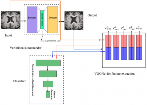
Considering MR images as input to the proposed model as depicted in Figure 1, which contains VAE as a major unit and their equivalent hippocampus segmentation is done at this stage.
We then extract features from the MRI and then use an improved version of the VAE for latent feature representation learning with the low-level features which are later used to train for classification tasks.
Figure 1. Simplified model for Alzheimer’s Disease classification
3.1 Extraction of shape features
Considering a baseline surface mesh Sr and a population of n surfaces{Si}i=1..n, spectral matching for every surface mesh as Si and Sr is accomplished as. Firstly, the initial map generation for the two surfaces is computed [20]. Then, according to Lombaert et al. [21], this initial map is utilized to create a smooth map for two surface meshes in the second stage. Vertices and nearby spots within every surface mesh are treated as vertices and edges of a graph in this case. Later, this group is then used to generate a graph Laplacian of each surface mesh. Finally, the Laplacian operator Li, in general, on each surface is demarcated as follows:
$L_i=G_i^{-1}\left(D_i-W_i\right)$ (1)
here, Wi is the weight matrix calculated from the measured distance of nodes that are connected. Here, Direfers to a diagonal matrix whose members are determined. Finally, Gi denotes the weighting matrix according to Shakeri et al. [22]. The spectral components are provided via the eigen decomposition of the Laplacian matrix Li. The final smooth map between two surfaces, Si and Sr, is created in the following phase, given an initial map c. The association graph is then given a Laplacian matrix, which generates an eigenvectors group to obtain two surface meshes.
In this VAE, the encoder E(x) job is to turn the image data into the same amount of latent vector data. Decoder D(z) task is to generate an output image. Finally, the pretrained VGGNetΦ(x) task extracts the relevant features needed for classification. In this current study, we use discriminator Dis(x) as a classifier for generating real and generated images. To increase classification accuracy, we applied VAE, which requires KL divergence loss $\mathcal{L}_{k l} \leftarrow D_{K L}(q(Z \mid X) \| p(Z))$ [23]. The other is a feature reconstruction loss. Explicitly, for a pre-trained network, Φ using input and output images and measuring the reconstruction loss of the lth hidden layer is expressed as $\mathcal{L}_{r e c}=\mathcal{L}^1+\mathcal{L}^2+\cdots+\mathcal{L}^l$, where denotes the feature reconstruction loss.
Rather than providing information to the discriminator, using the VGGNet as the discriminator's input is the better idea. The goal is to allow for more steady training while utilizing less information as feasible and employing a GAN model with pre-trained VGGNet architecture.
3.2 Neural network architecture
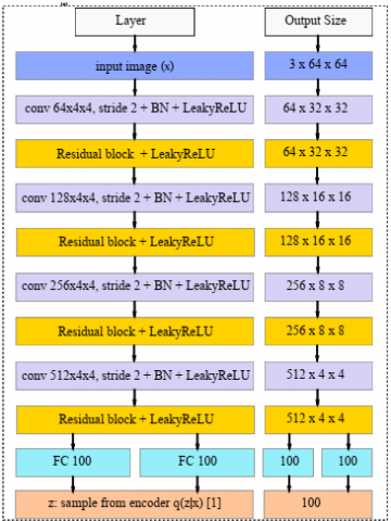
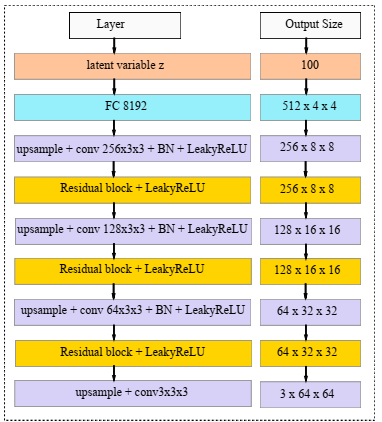
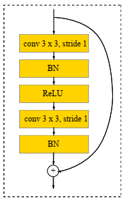
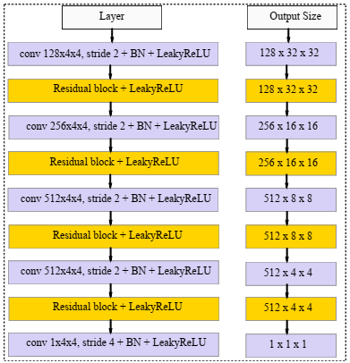
Both the autoencoder and discriminator networks, as illustrated in Figure 2, are deep residual CNNs based on Radford et al. [24]. By instead employing deterministic spatial functions like max-pooling, we build four convolutional layers in the encoder network with a 4×4 kernel and a 2×2 stride to accomplish spatial downsampling. Following each convolutional layer comes a batch normalizing and, for a gradient allowing, using LeakyReLU successively. After each convolutional layer, a residual block is added, and all of them comprise two 3×3 kernels of identical layers. Finally, the encoder includes two fully-connected layers (FCL) that will be utilized to compute the KL divergence loss and sample latent variable z. We employ 4 CLs with 3×3 kernels and 1×1 stride for the decoder. We also recommend that replicated padding be used instead of traditional zero-padding, such that the input map fill-out with the input edge replica. Every convolutional layer except the last one is covered by a residual layer, just like the encoder.
(a) Encoder
(b) Decoder
(c) Residual block
(d) Discriminator network
Figure 2. Simplified block diagram of encoder, decoder and discriminator network
We employ the nearest neighbor approach on a scale of 2 for upsampling rather than the partial stride convolution operation used by prior publications [25]. In addition, batch normalization is used to assist in stabilizing the entire training, and LeakyReLU is used as the activation function. DCGAN's architectural advancements inspire the discriminator's design. To accomplish spatial downsampling, we use convolutional layers with a 4×4 kernel and a 2×2 stride and append at the end of CL with a residual block. Later, discarding the sigmoid at last and stride CL of size 4×4 is employed for output incorporating a gradient of -0.01 and discriminator of 0.01.
3.3 Feature reconstruction loss
This is expressed as the mean squared error between feature representations in a DCNN as Φ. As in [26], we use VGGNet [27] as the loss network in our experiment. The primary idea of feature reconstructive loss is to search for evenness in the learnt feature space between real and generated images. Consider that Φl(x) represents the lth hidden layer. Φl(x) also signifies a block array of [Cl×Wl×Hl] dimensions. Clindicates the filter count, Wl means the width, and Hl denotes the height of the lth layer feature map. The squared Euclidean distance is a simple way to express the feature reconstruction loss (Ll) between two images (x and $\ddot{x}$).
$\mathcal{L}_l=\frac{1}{2 C_l W_l H_l} \sum_{c=1}^{c_l} \sum_{w=1}^{W_l} \sum_{h=1}^{H_l}\left(\Phi_l(x)_{c, w, h}-\Phi_l(\ddot{x})_{c, w, h}\right)^2$ (2)
Instead of merely using features from a single layer, we use visual information from many levels and integrate the VGGNet'soutputs. For example, the expression for the last reconstruction loss (RL) is calculated as follows:
$\mathcal{L}_{r e c}=\sum_{l=1}^L \frac{100}{C_l^2} \mathcal{L}_l$ (3)
where, $\mathcal{L}_l$ and Cl are the loss of features and filter count, and L is the total number of CLs of the model. In addition, to regulate the spread of the latent variable z, we use the KL divergence loss $\mathcal{L}_{kl}$ to regularize the encoder network. For training VAE accurately, we have to reduce KL divergence loss and reconstruction loss at every layer.
$\mathcal{L}_{\text {vae }}=\alpha \mathcal{L}_{k l}+\beta \mathcal{L}_{\text {rec }}$ (4)
where, α and β denote weighting values, respectively. It should be noted that VGGNet is solely utilized for feature extraction throughout the training process. In our current work, the MRI latent representation is the latent variable of the autoencoder.
3.4 Adversarial loss
In this, we added a VAE context to the GAN to generate the required outputs distributed throughout real images. WGAN is the basis of our adversarial training. To increase training stability even further, rather than directly feeding original images, we extracted features from the first layer of pretrained VGGNet and provided them to the discriminator. With the help of deep networks, to achieve a reconstructed image that is the same as the original. Later, the sigmoid is discarded, and 1 and -1 should be used as labels for real and generated images. We discovered that GAN can fail and that VAE is likely to take precedence when using too small labels, such as 1 and -1, during testing. Finally, as per Equation 5, our model may be trained end-to-end by adding three losses, and Algorithm 1 is used for the training approach.
$\mathcal{L}_{\text {vae }}=\alpha \mathcal{L}_{k l}+\beta \mathcal{L}_{\text {rec }}+\mathcal{L}_{G A N}$ (5)
where, $\mathcal{L}_{k l}$ denotes KL divergence loss, $\mathcal{L}_{r e c}$ denotes reconstruction loss and $\mathcal{L}_{G A N}$ denotes adversarial loss.
________________________________________________
Algorithm 1: Pseudo code for VAE-WGAN training model
________________________________________________
Input: feature parameter; Φ, pretrained model
WEncoder; WDecoder; WDiscriminator $\leftarrow$ Initialize parameters
repeat
X $\leftarrow$ mini-batch dataset images
$Z \leftarrow$ Encoder $(X)$
$\mathcal{L}_{k l} \leftarrow D_{K L}(q(Z \mid X) \| p(Z))$
$\widehat{\mathrm{X}} \leftarrow \operatorname{Decoder}(Z)$
$\mathcal{L}_{r e c} \leftarrow\|\Phi(\mathrm{X})-\Phi(\widehat{\mathrm{X}})\|^2$
$\mathcal{L}_{\text {GAN }} \leftarrow$ Discriminator $(X)-$ Discriminator $(\widehat{\mathrm{X}})$
$W_{\text {Encoder }} \stackrel{+}{\leftarrow}-\nabla_{W_{\text {Encoder }}}\left(\mathcal{L}_{k l}+\mathcal{L}_{\text {rec }}-\mathcal{L}_{\text {GAN }}\right)$
$W_{\text {Decoder }} \stackrel{+}{\leftarrow}-\nabla_{W_{\text {Decoder }}}\left(\mathcal{L}_{\text {rec }}-\mathcal{L}_{\text {GAN }}\right)$
$W_{\text {Discriminator }} \stackrel{+}{\leftarrow}-\nabla_{W_{\text {Disiminance }}}\,\,\,\,\,\,\, \mathcal{L}_{G A N}$
$W_{\text {Discriminator }} \leftarrow$ clip $\left(W_{\text {Discriminator }},-c, c\right)$
until convergence of parameters
_________________________________________
All the images are tested using the Anaconda tool. The proposed technique is evaluated using the Alzheimer's Disease Neuroimaging Initiative, a popular brain imaging dataset in Alzheimer's disease (ADNI: adni.loni.usc.edu). A subset of the most recent 1.5 T MR scans was used for this investigation. The left (label number 17) and right (label number 53) hippocampi were separated, and an automated segmentation process was used using commercial tools. Certain subjects are removed due to errors in the preprocessing stages. As a result, our study comprised 142 normal controls (NC), 83 Alzheimer's disease (AD) patients, 154 people with early MCI (EMCI), and 150 people with MCI (LMCI). There are four subfolders in the folder data (NC, AD, EMCI, LMCI). Every directory is divided into two sub-directories (17 and 53). All spectral meshes are stored in vtk format here. "data/NC/17/NC_1_17.vtk" represents the left hippocampus mesh of healthy subject 1, and "data/NC/53/NC 1_53.vtk" represents the right hippocampus mesh of the same subject.
4.1 Analysis of baseline and proposed work
Proposed work:The basic VAE uses per-pixel analysis, resulting in blurry outcomes since it sees images as "unstructured" input and each pixel is independent. The proposed study improves VAE performance by evaluating irregularity in deep feature space. Convolutional procedures allow pre-trained deep CNN to capture visual quality elements like spatial correlation. The adversarial loss is a "structured" measurement since GAN training involves high-level image classification, and no pixel is addressed separately.
Baseline: We train linear Support Vector Machines (SVM) with the same dataset after dimensionality reduction using principal components analysis (PCA) as a baseline. The features are extracted from surface meshes using spectral matching in the same manner as we recommended. In addition, SVM employs an optimal linear separating hyperplane to divide two data sets in a feature space. The ideal hyperplane is formed by increasing the minimal margin between the two sets. Consequently, the final hyperplane will rely only on boundary training patterns known as support vectors.
Six binary classification issues are considered here. Table 1 shows the results of all classes. We use 20% of the data for testing and the remaining 80% for training. For a fair review, the entire process is performed in five iterations.
Table 1. Performance comparison 3 metrics with a baseline and proposed method
|
Class |
Baseline (SVM) |
Proposed |
||||
|
Acc |
Sen |
Spe |
Acc |
Sen |
Spe |
|
|
NC/AD |
80 |
70 |
86 |
84 |
73 |
89 |
|
NC/EMCI |
55 |
52 |
58 |
56 |
52 |
60 |
|
NC/LMCI |
63 |
56 |
75 |
59 |
52 |
64 |
|
AD/EMCI |
76 |
65 |
71 |
81 |
70 |
82 |
|
AD/LMCI |
63 |
58 |
66 |
67 |
58 |
73 |
|
EMCI/LMCI |
51 |
50 |
52 |
63 |
62 |
66 |
Based on the trial findings, the regularization factor is 0.05. The classifier's performance is quantified in the analysis of the results by three metrics.
$\operatorname{Accuracy}(\mathrm{Acc})=\frac{\mathrm{TP}+\mathrm{TN}}{\mathrm{TP}+\mathrm{TN}+\mathrm{FP}+\mathrm{FN}}$ (6)
Sensitivity $($ Sen $)=\frac{\mathrm{TP}}{\mathrm{TP}+\mathrm{FN}}$ (7)
Specificity $($ Spe $)=\frac{\mathrm{TN}}{\mathrm{FP}+\mathrm{TN}}$ (8)
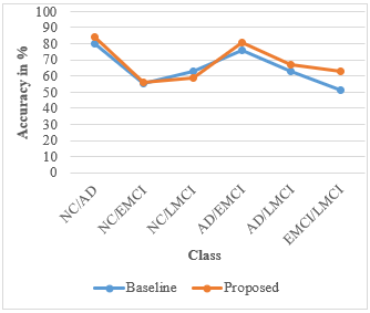
Figure 3 indicates that our proposed model is more accurate in most cases. As predicted, the highest classification accuracy is found for diagnostically highly differentiated groups. For example, 84% and 81% for the classification of NC versus AD and EMCI versus AD, respectively.
Figure 3. Performance comparison of accuracy for six classes for baseline and proposed work
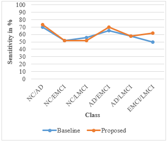
Figure 4 indicates that our proposed model generates greater sensitivity in most situations. As predicted, the highest sensitivity is achieved for diagnostically highly differentiated groups. For example, 73% and 70% of people agreed that NC was different from AD and that EMCI was different from AD.
Figure 4. Performance comparison of sensitivity for six classes for baseline and proposed work
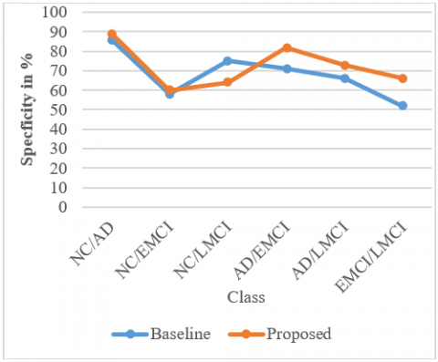
In particular, Figure 5 indicates that our proposed model generates higher specificity in most circumstances. As predicted, the highest specificity is achieved for diagnostically highly separated groups. For NC/AD, it is 89%, and AD/EMCI is 82%, respectively.
Figure 5. Performance comparison of specificity for six classes for baseline and proposed work
Table 2. Evaluation results of training data and test data with a baseline and proposed method
|
Evaluation metric |
Baseline |
Proposed |
||
|
Training Data (msec) |
Test Data |
Training Data |
Test Data |
|
|
ROC AUC |
0.8909 |
0.9175 |
0.9211 |
0.9322 |
|
Time (msec) |
250.109 |
167.68 |
189.21 |
145.71 |
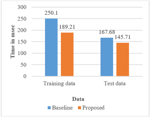
According to Table 2, the proposed model area under the receiver operating characteristic curve (ROC) curve for test data is 93.22%, and the testing time is 145.71 msec. The statistics table and ROC curve visualization summarize how the model generally works. For example, Figure 6 shows that baseline (SVM) performs poorly with a ROC AUC value of 91.75% and reconstructs very blurry images because of the shortcomings of per-pixel loss and consumes more time training time of 250.1 msec and a testing time of 167.68 msec. On the other hand, our proposed model incorporates VAE in the framework of GAN to produce outputs that exist on many natural images. This consumes less training time, 189.21 msec, and a testing time of 145.71 msec.
Figure 6. Comparison of the training and testing time using baseline and proposed model
This study presents a feature-learning technique for Alzheimer's disease classification based on a spectral feature representation and hippocampal morphology. Thus, extracted features from MRI are 3D surface meshes for node-to-node vertices using a spectral matching process. First, VAE is trained in hippocampal changes to generate the latent feature map. Then, for classification purposes, the SoftMax layer is used, and the dataset considered for this is the ADNI dataset. In addition, the proposed work mainly concentrated on AD/NC and EMCI/AD classes for the detection of various stages of dementia. The significance of VAE is shown by having less training and testing time compared to the baseline method for enhancing the diagnostic process. Other useful elements, including cognitive data and incorporating PET multimodal data, might be included in the future to improve classification accuracy.
[1] Jain, R., Jain, N., Aggarwal, A., Hemanth, D.J. (2019). Convolutional neural network based Alzheimer’s disease classification from magnetic resonance brain images. Cognitive Systems Research, 57: 147-159.https://doi.org/10.1016/j.cogsys.2018.12.015
[2] Gunawardena, K.A.N.N.P., Rajapakse, R.N., Kodikara, N.D. (2017). Applying convolutional neural networks for pre-detection of Alzheimer's disease from structural MRI data. In 2017 24th International Conference on Mechatronics and Machine Vision in Practice (M2VIP), Auckland, New Zealand, pp. 1-7. https://doi.org/10.1109/M2VIP.2017.8211486
[3] Sarraf, S., DeSouza, D.D., Anderson, J., Tofighi, G. (2017). DeepAD: Alzheimer’s disease classification via deep convolutional neural networks using MRI and fMRI. BioRxiv, 070441. https://doi.org/10.1101/070441
[4] McCrackin, L. (2018). Early detection of Alzheimer’s disease using deep learning. In Canadian Conference on Artificial Intelligence, pp. 355-359.https://doi.org/10.1007/978-3-319-89656-4_40
[5] Harris, P., Suarez, M.F., Surace, E.I., Méndez, P.C., Martín, M.E., Clarens, M.F., Tapajóz, F., Russo, M.J., Campos, J., Guinjoan, S.M., Sevlever, G., Allegri, R.F. (2015). Cognitive reserve and Aβ1-42 in mild cognitive impairment (Argentina-Alzheimer’s Disease Neuroimaging Initiative). Neuropsychiatric Disease and Treatment, 11: 2599. https://doi.org/10.2147/NDT.S84292
[6] Jack, C.R., Shiung, M.M., Gunter, J.L., O’brien, P.C., Weigand, S.D., Knopman, D.S., Boeve, B.F., Ivnik, R.J., Smith, G.E., Cha, R.H., Tangalos, E.G., Petersen, R.C. (2004). Comparison of different MRI brain atrophy rate measures with clinical disease progression in AD. Neurology, 62(4): 591-600. https://doi.org/10.1212/01.WNL.0000110315.26026.EF
[7] Fang, C., Li, C., Cabrerizo, M., Barreto, A., Andrian, J., Rishe, N., Loewenstein, D., Duara, R., Adjouadi, M. (2018). Gaussian discriminant analysis for optimal delineation of mild cognitive impairment in Alzheimer’s disease. International Journal of Neural Systems, 28(8): 1850017. https://doi.org/10.1142/S012906571850017X
[8] Lombaert, H., Criminisi, A., Ayache, N. (2015). Spectral forests: Learning of surface data, application to cortical parcellation. In International Conference on Medical Image Computing and Computer-Assisted Intervention, pp. 547-555. https://doi.org/10.1007/978-3-319-24553-9_67
[9] Eschenburg, K.M., Grabowski, T.J., Haynor, D.R. (2021). Learning cortical parcellations using graph neural networks. Frontiers in Neuroscience, 15. https://doi.org/10.3389/fnins.2021.797500
[10] Lombaert, H., Sporring, J., Siddiqi, K. (2013). Diffeomorphic spectral matching of cortical surfaces. In International Conference on Information Processing in Medical Imaging, pp. 376-389. https://doi.org/10.1007/978-3-642-38868-2_32
[11] Lopez, R., Boyeau, P., Yosef, N., Jordan, M., Regier, J. (2020). Decision-making with auto-encoding variational Bayes. Advances in Neural Information Processing Systems, 33: 5081-5092.
[12] Hu, M.F., Zuo, X., Liu, J.W. (2022). Survey on deep generative model. Acta Automatica Sinica, 48: 40-74. https://doi.org/10.16383/j.aas.c190866
[13] Gordon, J., Hernández-Lobato, J.M. (2020). Combining deep generative and discriminative models for Bayesian semi-supervised learning. Pattern Recognition, 100: 107156. https://doi.org/10.1016/j.patcog.2019.107156
[14] Hua, G., Chen, D.D. (2022). Chapter 5 - Deep conditional image generation: Towards controllable visual pattern modeling. Advanced Methods and Deep Learning in Computer Vision, 191-219. https://doi.org/10.1016/B978-0-12-822109-9.00014-X
[15] An, N., Ding, H., Yang, J., Au, R., Ang, T.F. (2020). Deep ensemble learning for Alzheimer's disease classification. Journal of Biomedical Informatics, 105: 103411. https://doi.org/10.1016/j.jbi.2020.103411
[16] Jia, H., Wang, Y., Duan, Y., Xiao, H. (2021). Alzheimer’s disease classification based on image transformation and features fusion. Computational and Mathematical Methods in Medicine, 1-11. https://doi.org/10.1155/2021/9624269
[17] So, J.H., Madusanka, N., Choi, H.K., Choi, B.K., Park, H.G. (2019). Deep learning for Alzheimer’s disease classification using texture features. Current Medical Imaging, 15(7): 689-698. https://doi.org/10.2174/1573405615666190404163233
[18] Shanmugam, J.V., Duraisamy, B., Simon, B.C., Bhaskaran, P. (2022). Alzheimer’s disease classification using pre-trained deep networks. Biomedical Signal Processing and Control, 71: 103217. https://doi.org/10.1016/j.bspc.2021.103217
[19] Liang, C., Lao, H., Wei, T., Zhang, X. (2022). Alzheimer’s disease classification from hippocampal atrophy based on PCANet-BLS. Multimedia Tools and Applications, 81(8): 11187-11203. https://doi.org/10.1007/s11042-022-12228-0
[20] Lombaert, H., Grady, L., Polimeni, J.R., Cheriet, F. (2012). FOCUSR: Feature oriented correspondence using spectral regularization--a method for precise surface matching. IEEE Transactions on Pattern Analysis and Machine Intelligence, 35(9): 2143-2160. https://doi.org/10.1109/TPAMI.2012.276
[21] Lombaert, H., Sporring, J., Siddiqi, K. (2013). Diffeomorphic spectral matching of cortical surfaces. In International Conference on Information Processing in Medical Imaging, pp. 376-389. https://doi.org/10.1007/978-3-642-38868-2_32
[22] Shakeri, M., Lombaert, H., Datta, A.N., et al. (2016). Statistical shape analysis of subcortical structures using spectral matching. Computerized Medical Imaging and Graphics, 52: 58-71. https://doi.org/10.1016/j.compmedimag.2016.03.00
[23] Lopez, R., Regier, J., Jordan, M.I., Yosef, N. (2018). Information constraints on auto-encoding variational bayes. Advances in Neural Information Processing Systems, 31.
[24] Radford, A., Metz, L., Chintala, S. (2015). Unsupervised representation learning with deep convolutional generative adversarial networks. arXiv preprint arXiv:1511.06434.
[25] Shelhamer, E., Long, J., Darrell, T. (2016). Fully Convolutional Networks for Semantic Segmentation. IEEE Transactions on Pattern Analysis and Machine Intelligence, 39: 1-1. https://doi.org/10.1109/TPAMI.2016.2572683
[26] Gatys, L.A., Ecker, A.S., Bethge, M. (2015). A neural algorithm of artistic style. arXiv preprint arXiv:1508.06576. https://doi.org/10.1167/16.12.326
[27] Simonyan, K., Zisserman, A. (2014). Very deep convolutional networks for large-scale image recognition. arXiv preprint arXiv:1409.1556. https://doi.org/10.48550/arXiv.1409.1556