Marwa Jamal* | Tariq A. Hassan
© 2022 IIETA. This article is published by IIETA and is licensed under the CC BY 4.0 license (http://creativecommons.org/licenses/by/4.0/).
OPEN ACCESS
Recently, data of multimedia performs an exponentially blowing tendency, saturating daily life of humans. Various modalities of data, includes images, texts and video, plays important role in different aspects and has wide. However, the key problem of utilizing data of large scale is cost of processing and massive storage. Therefore, for efficient communications and for economical storage requires effective techniques of data compression to reduce the volume of data. Speech coding is a main problem in the area of digital speech processing. The process of converting the voice signals into a more compressed form is speech coding. In this work, we demonstrate that a DCT with a chaotic system combined with run-length coding can be utilized to implement speech coding of very low bit-rate with high reconstruction quality. Experimental result show that compression ratio is about 13% when implemented on Librispeech dataset.
speech coding, data compression, transform coding, neural speech coding, speech signal
Process of speech coding quantizes voice signal to a more compact bitstream for efficient storage and transmissions in systems of telecommunication. Speech codecs are designed to address the tradeoff between high perceptual quality, low bitrates, low complexity, delays, …etc. Speech codecs are categorized into two classes, waveform, and vocoder coders. To model, the production process of human vocoders utilizes a few parameters, such as pitch frequency, vocal tracts, etc. In contrast, to make the reconstructed voice similar to the input voice signal coders of waveform compress and reconstruct it as “perceptually” as possible. Waveform coder supports a bitrates of wide range with scalable performance and is more potent to noise, while conventional vocoders can encode voice at low bitrates and are efficient computationally [1].
Data compression applications are pervasive: real-time music and live videos across the planet, storing thousands of songs and images on a tiny single drive, and more. Enhanced compression in some ways, is what made these innovations possible in the first place, and building better and more efficient compression methods might help them spread even [2].
The main purpose of this study is to utilize a compression approach that decreases the quantity of lost information in the voice signal to some level. As a result, the suggested method's design will emphasize lossless compression while simultaneously ensuring that the compressed data is as small as feasible to achieve a high compression rate [3].
The rest of the paper is arranged as follows, Section 2 described the literature review, Section 3 presents the Theoretical background, Section 4 illustrates the proposed method, whereas the experimental result is presented in Section 5, and Section 6 represents the conclusion.
Several methods with various performance amounts have been utilized in the last few years. The most popular audio coders are depending on using one of the two techniques (sub-band coding and transform coding). Transform coding uses a mathematical transformation like Discrete Cosine Transform (DCT) and Fast Fourier Transform (FFT), Sub-band coding divides the signal into several sub-bands, using a band-pass filter [4]. The system [3] suggests using the JPEG method for the audio signal which uses the DCT method in its process to transform the domain of the signal and then compress the signal by the quantization process.
One of the powerful speech analysis techniques is the method of linear predictive analysis. The main idea of LPC is that the sample of voice can be approximated as a linear combination of previous samples. Al-azawi and Drweesh [4] implemented a voice excited LPC vocoder for low bit rate speech compression.
Sharma [5] implemented audio compression using run-length coding (RLE) and Huffman. The sampling frequency is calculated in preprocessing step from the audio file. After preprocessing step dynamic Huffman and RLE coding is implemented. The objective of the author is to obtain less Time Elapsed to compress and the utmost possible compression.
Existing research on the processing and efficient compression of DNNs can be classified into three categories, based on their design levels, software algorithms, hardware platforms, and memory technologies. Patil and Kulat [6] introduce a unique integer-adder deep neural network that in speech improvement accelerates the inference process and compresses the size of the model, a major task in the processing of voice-signal, by replacing the floating-point multiplier with an integer-adder.
The way that section titles and other headings are displayed in these instructions, is meant to be followed in your paper.
3.1 Discrete Cosine transforms (DCT)
DCT, presented first in 1974, has gained a lot of traction in recent years. It is widely used due to its optimal performance, DCT is implemented especially in voice compression, utilized in the image analysis, and signal processing due to its good performance. DCT converts an input signal from the time domain to the frequency domain, and its 1D version is useful for examining 1D signals such as voice signals. DCT is consisting of (AC) and (DC) coefficients, in which the (DC) holds the average signal value and is coefficient C (0), whereas the rest coefficients are referred to as the AC coefficients [7].
$C(u)=a(u) \sum_{i=0}^N s(i) \cos \left(\frac{u \pi(2 i+1)}{2 N}\right)$ (1)
$a(u)=\left\{\begin{array}{l}\sqrt{1 / N} \text { if } u=0 \\ \sqrt{2 / N} \text { if } u \neq 0\end{array}\right.$ (2)
3.2 Quantization
The process of quantization is the representation of a large set of values with a much smaller set. A simple quantization method would be to illustrate all the source products with the integer value closest to them. A group of consecutive data is quantized to a data group of discrete values. The primary purpose is to reduce the amount of data in threshold coefficients [8].
3.3 Run-length coding
RLE is a lossless data compression method. RLE compresses data by minimizing repeat and sequential called runs. It does this by recording the number of runs, followed by the data. For processing, individual channel matrices were extracted and employed. Firstly, each matrix was examined row by row for specifying repeating pixels. The pixel value and frequency of recurrence were then used to replace each set of such repeats. The pixel value and frequency of recurrence were then used to replace each set of such repeats. This was implemented exhaustively throughout the matrix. The frequency was not used for a single occurrence of a given value since it would produce an overhead that would reduce compression performance [9].
3.4 Logistic chaotic map
A logistic function is used to drive the logistic map, which is utilized to define some species' quantity changing procedure. It is illustrated as follows: [10]
$X_{n+1}=\mu X_n\left(1-X_n\right)$ (3)
here, 0< Xn <1, and the parameter P has the range limitation as [3.569946 and 4.0]. When P is in the range, the logistic map will lead to chaos, the other way round, when P is out of the range, Eq. (3) will not produce chaos. A chaotic series must be produced by chaos, so P must be in the range of [3.569946, 4] when a logistic map is utilized to produce chaotic series.
3.5 Gauss chaotic map
Every chaotic map contains essential properties like deterministic, simple to produce, and difficult to calculate. Gauss iterated map is one such kind of chaotic map [11]. The fundamental attributes of the Gauss map which make it distinct from a logistic map are:
The generalized Gauss map has an operation of a single dimension. It is a nonlinear iterated map of the reals into the real interval as produced by the gaussian function [12].
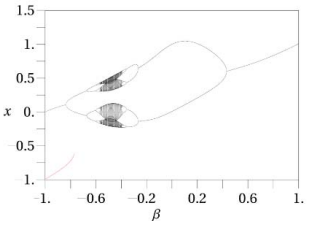
$X_{N+1}=\exp \left(-a X_2^N\right)+\beta$ (4)
By taking ∝= 4.9 and ß= [-1, +1] values, Figure 1 show the Gauss iterated map.
Figure 1. Gaussian map
3.6 Performance evaluation
Compression ratio is conducted to measures the overall performance of the suggested speech compression system. Compression factor (C) is used to assess the reconstructed signal's performance [13].
$C=\frac{\text { length of orginal signal }}{\text { length of compressed signal }}$ (5)
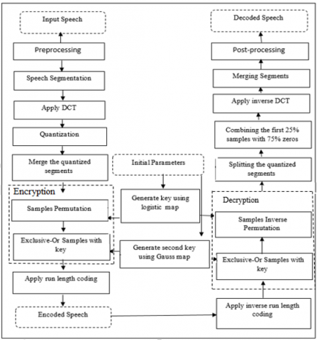
The suggested speech compression system, which is consisted of encoding and decoding, is explained in detail in the following subsections. The block diagram of suggested speech encoding and decoding is illustrated in Figure 2.
4.1 Encoding
Encoding consist of many stages which are used altogether for reduction of the required audio data size reduction and to represent the audio data in compressed form. The stages implemented for the encoding are:
(1) Load samples of speech data, the speech signal is demonstrated by the 1D array.
(2) Please do not include captions as part of the figures or put them in “text boxes”. Preprocessing stages which are responsible for speech signal framing and then solving the problem of silence gaps by calculating the energy of each frame depend on the following formula:
$E(m)=\sum_{n=1}^N x_m(n)^2$ (6)
A vector is used consisting of values either 1 or 0 to indicate frame energy depending on the threshold value. The frame with high energy is translated into a new vector.
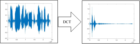
(3) DCT is applied to each segment to decompose it separately. The Eqns. (1) and (2) are applied to obtain a set of DCT coefficients. The output of DCT coefficients are real values, and before compression, each segment must be quantized to increase the compression. Figure 3 illustrate an example of DCT.
Figure 2. Block diagram of the proposed system (encoding and decoding)
Figure 3. Example of DCT process
(4) Quantization is applied to each segment and some coefficients are eliminated from the beginning of the segment. The ratio of the eliminated parts could be 20 to 30 percent of the segment. Then segments are merged into a new vector. The value of the produced vector is rearranged to make it ready for the next stage.
(5) At this stage logistic map is employed to generate the key used in the permutation stage. Key is generated using Eq. (3).
(6) Sample permutation stage is involved rearranging the sample using a key generated from the previous stage. Then sample values are rounded to prepare them for the next stage. Table 1 illustrates an example of the permutation process.
Table 1. Permutation numbers for samples
|
# |
Generated numbers |
Key index |
Sorted numbers |
|
1 |
0.814724 |
6 |
0.09754 |
|
2 |
0.905792 |
3 |
0.126987 |
|
3 |
0.126987 |
11 |
0.157613 |
|
4 |
0.913376 |
7 |
0.278498 |
|
5 |
0.632359 |
8 |
0.546882 |
|
6 |
0.09754 |
5 |
0.632359 |
|
7 |
0.278498 |
1 |
0.814724 |
|
8 |
0.546882 |
2 |
0.905792 |
|
9 |
0.957507 |
4 |
0.913376 |
|
10 |
0.964889 |
9 |
0.957507 |
|
11 |
0.157613 |
10 |
0.964889 |
|
12 |
0.970593 |
12 |
0.970593 |
(7) At this stage, the gauss map is utilized to generate a key by using Eq. (4) for each sample.
(8) An XOR process is performed between each sample and its corresponding key generated from the Gauss map to obtain an encrypted sample.
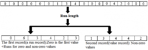
(9) Long runs of zero-symbols are coded to produce streams of small integers. RLE has solved this issue that replacing symbols of long runs of zero with a count of run length and non-zero samples. An example of the RLE process is illustrated in the Figure 4.
Figure 4. Example of run length coding
4.2 Decoding
Decoding is similar, but the process is built-in an inverted sequence. A reconstructed speech signal version is obtained from the decoded speech signal. The stages of decoding are: i) inverse RLE, ii) Exclusive-0r samples with key, iii) inverse sample permutation, iv) splitting the quantized segments, v) De-quantization, vi) inverse DCT, vii) merge segments, viii) post-processing.
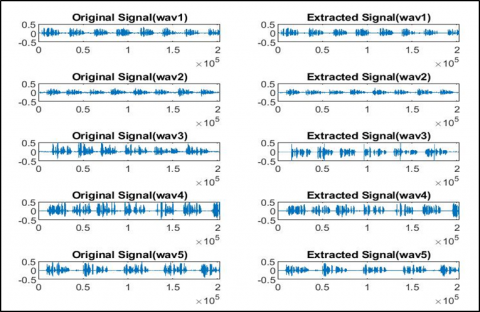
The proposed system has experimented on the Librispeech dataset. Randomly selected five speech files of type (.wav) and (mono) of length (25.4) sec to test the system. Figure 5 describes the original signal and the decoded signal.
Figure 5. Original and extracted speech signal
In the first stage, the signal is segmented into fixed-length frames of a length of 30 msec, and energy is calculated for each frame. The frame with energy higher than the threshold is set to one and otherwise zero. Only frames with high energy are kept for the next stage. Table 2 illustrates the amount of reduction and compression rate at this stage.
The speech signal extracted from the first stage is set in a new vector. In this stage, Segment a speech signal into frames of 1 sec each of (8,000) samples. Perform DCT on each frame, and eliminates 25% percent of each frame at the quantization step. A new vector is built from the signal generated from the quantization step. To implement the encryption process permutation is performed based on a key generated from a logistic map and the XOR process is performed on the result with a key generated from a gauss map. Then the result is transformed into binary one column of bits (0, 1) to prepare it for run-length coding.
RLE is removing zero and one while keeping only the length of them in which the first value refers to the number of ones and the next to the number of zeros in the stream and so on. Reduction in RLE is illustrated in Table 3. The compression ratio and final number of bits are shown in Table 4. In this work, two chaotic maps are used to generate the keys used in the permutation and XOR process.
Logistic and Gaussian maps are employed. Chaotic maps showed good random proportions, as illustrated in Table 5.
Table 2. Reduction in preprocessing step
|
No. of Samples |
Size in Bye |
||||
|
Original wave |
Preprocessed wave |
Noof Frames |
Original way in bytes |
Preprocessed wave in bytes |
Compression Rate |
|
203200 |
106320 |
443 |
406400 |
212640 |
52.32% |
|
203200 |
116880 |
487 |
406400 |
233760 |
57.52% |
|
203200 |
108960 |
454 |
406400 |
217920 |
53.62% |
|
203200 |
105360 |
439 |
406400 |
210720 |
51.85% |
|
203200 |
103440 |
431 |
406400 |
206880 |
50.91% |
Table 3. Reduction in size of run-length encoding
|
Preprocessed |
Padding zero |
Size in bit |
RLE |
Remove (0, 1) RLE |
Size in bit |
|
106320 |
112000 |
1792000 |
452852 |
226426 |
452852 |
|
116880 |
120000 |
1920000 |
483126 |
241563 |
483126 |
|
108960 |
112000 |
1792000 |
452110 |
226055 |
452110 |
|
105360 |
112000 |
1792000 |
449602 |
224801 |
449602 |
|
103440 |
104000 |
1664000 |
416982 |
208491 |
416982 |
Table 4. Compression ratio
|
The size of wave files in bits =203200*16=3251200 |
|||||
|
Size in bit |
452852 |
483126 |
452110 |
449602 |
416982 |
|
Compression ratio |
0.139288 |
0.148599 |
0.139059 |
0.138288 |
0.128255 |
Table 5. Chaotic map test
|
Test |
P-value |
Test |
P-value |
Status |
|
Run test |
0.10113399 |
Maurer’s universal statistical |
3.83166E-05 |
pass |
|
Serial test |
0.025637988 |
longest run of ones in the block test |
0.00107981 |
Pass |
|
Random excursion variant test |
0.623482916 |
Linear complexity |
0.690011 |
Pass |
|
random excursion |
0.711602856 |
Frequency test within a block test |
0.033940472 |
pass |
|
Non-overlapping template matching |
0.811286216 |
Discrete Fourier Transform test |
0.715176994 |
Pass |
|
Frequency monobit |
0.003089315 |
Cumulative sum test |
0.004274442 |
Pass |
In this work, we proposed a speech coding model based on DCT and RLE based on a chaotic map for lossless compression. The suggested system is implemented on five speech samples from Librispeech dataset. Experimental results show that the proposed system significantly improved the coding efficiency and achieved a compression ratio of about 13% which is supposed to be a good result in speech coding. The proposed system reduced speech signal size and avoided the requirement for much storage. The conducted test result showed that the suggested system is promising. The following stimulated remarks are summarized: i) The suggested compression system utilizing the DCT and RLE method indicate acceptable compression ratio while maintaining the quality of speech signal as illustrated in Table 4, ii) RLE reduced the physical size of repeated consecutive values.
|
a(u) |
AC coefficients |
|
C(u) |
DC coefficients |
|
C |
Compression ratio |
|
RLE |
Run length encoding |
|
DCT |
Discrete cosine transform |
|
Greek symbols |
|
|
a |
alpha |
|
b |
beta |
|
µ |
mean |
[1] Zhen, K., Lee, M.S., Sung, J., Beack, S., Kim, M. (2017). Efficient and scalable neural residual waveform coding with collaborative quantization. ICASSP 2020 - 2020 IEEE International Conference on Acoustics, Speech and Signal Processing (ICASSP), pp. 361-365. https://doi.org/10.1109/ICASSP40776.2020.9054347
[2] Kankanahalli, S. (2018). End-to-end optimized speech coding with deep neural networks. 2018 IEEE International Conference on Acoustics, Speech and Signal Processing (ICASSP), pp. 2521-2525. https://doi.org/10.1109/ICASSP.2018.8461487
[3] Hassan, T.A., Al-Hashemy, R.H., Ajel, R.I. (2020). Speech signal compression algorithm based on the jpeg technique. Journal of Intelligent Systems, 29(1): 554-564. http://dx.doi.org/10.1515/jisys-2018-0127
[4] Al-azawi, R.J., Drweesh, Z.T. (2019). Compression of audio using transform coding. Journal of Communications, 14(4): 301-306. https://doi.org/10.12720/jcm.14.4.301-306
[5] Sharma, N. (2012). Speech compression using linear predictive coding (LPC). International Journal of Advanced Research in Engineering and Applied Sciences, 1(5): 16-28.
[6] Patil, R.B., Kulat, K.D. (2017). Audio compression using dynamic Huffman and RLE coding. 2017 2nd International Conference on Communication and Electronics Systems (ICCES), pp. 160-162. https://doi.org/10.1109/CESYS.2017.8321256
[7] Lin, Y.C., Hsu, Y.T., Fu, S.W., Tsao, Y., Kuo, T.W. (2019). IA-NET: Acceleration and compression of speech enhancement using integer-adder deep neural network. INTERSPEECH, pp. 1801-1805. http://dx.doi.org/10.21437/Interspeech.2019-1207
[8] Ahmed, Z.J., George, L.E., Hadi R.A. (2021). Audio compression using transforms and high order entropy encoding. International Journal of Electrical and Computer Engineering, 11(4): 3459-3469. http://dx.doi.org/10.11591/ijece.v11i4.pp3459-3469
[9] Manohar, P.K.R., Pratyusha, M., Satheesh, R., Geetanjali, S., Rajasekhar, N. (2015). Audio compression using Daubechie wavelet. IOSR Journal of Electronics and Communication Engineering (IOSR-JECE), 10(2): 41-44. https://doi.org/10.9790/2834-10234144
[10] Chakraborty, D., Banerjee, S. (2011). Efficient lossless colour image compression using run length encoding and special character replacement. International Journal on Computer Science and Engineering (IJCSE), 3(7): 2719-2725.
[11] Zhang, J., Zhu, Y.X., Zhu, H.P., Cheng, J. (2017). Some improvements to logistic map for chaotic signal generator. 3rd IEEE International Conference on Computer and Communications, pp. 1090-1093. https://doi.org/10.1109/CompComm.2017.8322711
[12] Sahay, A., Pradhan, C. (2017). Multidimensional comparative analysis of image encryption using gauss iterated and logistic maps. International Conference on Communication and Signal Processing, pp. 1347-1351. https://doi.org/10.1109/ICCSP.2017.8286603
[13] Vig, R., Chauhan, S.S. (2018). Speech compression using multi-resolution hybrid wavelet using DCT and Walsh transforms. Procedia Computer Science, 132: 1404-1411. https://doi.org/10.1016/j.procs.2018.05.070