Achmad Rizal* | Vivi Aliyah Putri Handzah | Purba Daru Kusuma
© 2022 IIETA. This article is published by IIETA and is licensed under the CC BY 4.0 license (http://creativecommons.org/licenses/by/4.0/).
OPEN ACCESS
The heart sound coming from the patient is observed using a stethoscope, which is a medical tool to determine the patient's condition. The technique for this observation is called auscultation. This sound describes the condition of a person's heart. Because auscultation relies on the experience and knowledge of doctors, various methods for analyzing heart sounds are automatically developed by researchers. In this study, a method for classifying normal heart sounds and murmurs is proposed using the grey-level difference matrix (GLDM) feature taken from the short-time Fourier transform (STFT) plot. The STFT plot is converted into an image then the GLDM characteristics are calculated as input for the support vector machine as a classification. The experimental result shows that the highest accuracy of 83% is achieved using STFT 200-100 in four directions of GLDM. Even though this accuracy is not as high as the previous research, the proposed method is still open for exploration, such as distance selection in GLDM or other image analysis methods.
grey-level difference matrix, short-time Fourier transform, auscultation, classification
Stethoscope is used by medical personnel to listen to acoustic signals from inside the human organs [1]. When diagnosing, the body parts that are examined are the lungs, heart, and intestines. The type and intensity of the acoustic signal produced help medical personnel to diagnose of the patient's condition [2]. A stethoscope is a must-have tool because of its essential role in diagnosing a patient's disease. In the current observation process, the technique for listening to the sounds from inside the patient's body is called auscultation [3]. This process uses a stethoscope to get a more precise sound. However, there are many obstacles due to this direct approach. These problems are low frequency, low amplitude, environmental noise, hearing sensitivity, and sounds with almost identical patterns.
One of the signals heard using the auscultation technique is heart sound. By listening to this sound, doctors diagnose abnormalities in the heart. Considering these subjective factors, many methods have been developed to classify heart sounds automatically using digital signal processing method [4].
In general, heart sound signal processing can be divided based on the signal domain: time domain, frequency domain, and time-frequency domain [5]. Signal processing in the time-domain, for example, calculating statistical features on heart sounds, empirical mode decomposition (EMD), and fractal dimensions [6]. Meanwhile, heart sound signal processing in the frequency domain includes filter bank, mean-power of frequency band, MFCC, quartile frequency, and zero-crossing analysis [7]. Signal processing in the frequency domain mainly involves Fourier transforms to convert the signal from the time domain to the frequency domain. Heart sound signal processing in the time-frequency domain, such as short-time Fourier transform (STFT), Wigner-Ville distribution (WVD), Stockwell transform (S-Transform), Hilbert-Huang Transform (HHT), or wavelet transforms [5]. The use of the time-frequency domain is quite widespread because this method provides information about the frequency component of the signal at each time.
Because the previously mentioned time-frequency domain method only changes the signal from the time domain to the time-frequency domain, it is still necessary to use a feature extraction method to obtain the characteristics of the signal. One of the methods is signal complexity. Wang et al. used wavelet-time entropy to separate normal and abnormal heart sound signals [8]. Other researchers have used the fractal dimension to distinguish normal heart sounds and murmurs [9]. Short-time Fourier transform (STFT) as a method for transforming 1D signals to the time-frequency domain was also used in previous studies. STFT and tensor decomposition were proposed by Zhang et al. as characteristics of normal and abnormal heart sounds [10]. Meanwhile, wavelet entropy is used as a feature of STFT from unsegmented signals from heart sounds [11]. From all previous studies, characteristics were calculated directly on the STFT; no analysis was carried out on the distribution of information on the STFT.
This study proposes a novel method for classifying normal and abnormal heart sounds using STFT and Gray level difference method (GLDM) as feature extraction method. STFT was used to change the time domain to the time-frequency domain [12]. Then, the GLDM texture analysis method analyzes heart sounds [13]. Heart sound, a 1D signal, is transformed into 2D using STFT and then analyzed using GLDM. GLDM is a feature extraction method to see an image's texture by creating a new image, which is the absolute value of the difference between two pixels at a certain distance and direction. Because it is calculated from the absolute value of the difference between two pixels, GLDM produces a new image whose texture can be observed. Then, some statistical parameters are calculated. This is different from other texture analysis methods, such as gray-level co-occurrence matrix (GLCM) and gray level rung-length (GLRL) [14]. The GLCM calculation does not produce a new image but creates a co-occurrence matrix, which is the result of calculating the number of occurrences with a pixel value at a certain distance. Meanwhile, GLRL generates a run-length encoding code that describes the pixel value and its repetition [15]. The results of GLCM and GLRL are not images, so they cannot be assessed visually directly. This proposed method hopefully becomes a biological signal processing method alternative that will be obtained by utilizing spatiotemporal information from the signal.
The remainder of this paper is structured as follows. The proposed method is explained in section two. Then, the experiment, result, findings, and more profound analysis are discussed in section three. At the end of our paper, we present the conclusion and future research potential in section four.
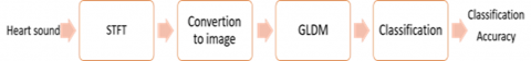
The proposed method is as shown in Figure 1. The STFT process is used for heart sounds to produce a spectrogram. The spectrogram is then converted into an image. Then, the GLDM process is carried out with a specific distance d. Five features of GLDM are calculated from the image and used as input for support vector machine (SVM) as classifier to determine whether the heart sound is normal or abnormal. The following subsections describes detail of each process.
2.1 Heart sound database
The heartbeat makes two separate noises, which are commonly referred to as lub-dub. The lub sound is produced by the tricuspid and mitral (atrioventricular) valves, which prevent backflow of blood from the atria (auricles) to the ventricles (heart chambers) (1). The first cardiac sound (S1) is a sound that appears practically concurrently with the commencement of the QRS complex on an ECG and occurs before systole (the period when the heart contracts). The second heart sound is referred to as the dub sound (S2). The semilunar (aortic and pulmonary) valves that discharge blood into the pulmonary and systemic circulation systems close, causing it. Before the atrioventricular valve reopens, this valve closes at the conclusion of systole. This S2 sound occurs practically concurrently with the electrocardiogram's T wave's termination. The third heart sound (S3) corresponds to the cessation of atrioventricular filling, whereas the fourth heart sound (S4) correlates with atrial contraction. This S4 sound has a low amplitude and low-frequency component [16].
As in earlier studies [9] the heart sound data set is separated into two categories: normal and pathological. Physionet.org provided 50 normal sounds and 50 murmurs as input data [17-19]. The image of the heart sound is shown in Figure 2.
Figure 1. Diagram block of proposed method
Figure 2. (a) Normal heart sound (b) Murmur
The amplitude normalization process is carried out to reduce the variation due to the difference in the heart sound amplitude. It is formalized as (1) and (2):
$y(n)=x(n)-\frac{1}{N} \sum_{i=1}^{N} x(i)$ (1)
$y(n)=\frac{x(n)}{\max |x|}$ (2)
where, the input signal is x(n) and the output signal is y(n).
2.2 Short-Time Fourier Transform (STFT)
Signals are transformed from the time domain to the time-frequency domain using the STFT or spectrogram method. At a specific time interval, this algorithm will segment the signal. FFT is used to translate the segmented signal into the frequency domain. The mathematical expression of STFT is shown in Eq. (3) [18].
$X_{S T F T}[m, n]=\sum_{k=0}^{L-1} x[k] g[k-m] e^{-j 2 \pi n k / L}$ (3)
where, x(k) is the signal and g(k) is the L-point window. So STFT can be said as a Fourier transform of the x(k) signal windowed using g(k).
In this study, several parameters were used in the STFT used as in [20] as follows:
2.3 Feature extraction using GLDM
Grey-level difference matrix (GLDM) is the difference between adjacent pixels proposed by Weszka et al. [13] for the characterization of an image. To observe the intensity fluctuation in an image, Weszka et al. employed the absolute value of the difference between two neighboring pixels in the horizontal, vertical, and diagonal axes [13].
The number of adjacent pixels in the direction θ is represented by H(θ) that has g as absolute difference between two pixels. Where it is the probability of adjacent pixels in the direction θ to the absolute value of the difference g. GLDM’s features of the image is calculated as follows:
Gradient contrast:
$G C=\sum_{g} g^{2} h(g l \theta)$ (4)
Gradient second moment:
$G S M=\sum_{g}[h(\theta)]^{2}$ (5)
Gradient entropy:
$G E=-\sum_{g} h(g l \theta) \log h(g l \theta)$ (6)
Gradient mean:
$G M=\sum_{g} h(g l \theta) g$ (7)
Inverse-difference moment:
$I D M=\sum_{g} \frac{h(g l \theta)}{\left(g^{2}+1\right)}$ (8)
In this study, the five features were calculated in the directions of 0°, 45°, 90°, and 135°.
2.4 Support Vector Machine (SVM)
SVM is used as a classifier. It uses a hyperplane to divide data into two classes. The data nearest to the hyperplane is referred to as the support vector. The gap between the hyperplane and the super vector is called the margin. The SVM algorithm relies on the most significant margin between the hyperplane and the super vector. It is dependent on the optional hyperplane to get the maximum margin. Finding the proper hyperplane is critical for SVM classification accuracy [16].
The basic classification technique divides heart sound data into two classes, normal and murmur, using a linear hyperplane. In other cases, it is unable to classify some data appropriately. The kernel function is another SVM solution for solving distinct data more successfully than linear hyperplane [17]. Linear, quadratic, and cubic kernel functions were used in this investigation. Linear kernel is used as the kernel algorithm because its function is the simplest and is typically like a non-kernel counterpart. The inner product (xi, xj) with an optional constant c gives it. The linear kernel function is formalized in (9):
$k\left(x_{i}, x_{j}\right)=x_{i}^{T} x_{j}+c$ (9)
Figure 3 shows a spectrogram of normal heart sounds and murmurs using a 500-475 STFT with 512 NFFT. It shows that there is a difference between the spectrogram of normal heart sounds and heart murmurs. This difference will be quantized by GLDM and then classified. In Figure 3, cuts are made at high frequencies, assuming that information on heart sounds is concentrated at frequencies < 250 Hz. Even though the assumption is that the frequency is concentrated below 250, the STFT plot is cut at a frequency of 500 Hz; this is to anticipate if there is a frequency component above 250. From the frequency spectrum of the two types of normal heart sounds and murmur, we can see that the dominant frequency is below 250 Hz, but there is still some small frequency above 250 Hz. The method used is not intended to detect the presence of frequencies above 500 Hz but to see the pattern of signal fluctuations in the time and frequency domains represented by the texture of the STFT image. Two images of the heart sound spectrum, normal and murmur, are provided in Figure 4.
Figure 5 shows the converted image from Figure 3. The difference can be seen in the distribution of the black color obtained. This black and white distribution will be processed using GLDM, and the GLDM characteristics will be calculated as input from SVM as a classifier.
Figure 3. (a) Spectrogram of normal heart sound; (b) Spectrogram of murmur heart sound
Figure 4. (a) Frequency spectrum of normal sound; (b) Frequency spectrum of murmur sound
Figure 5. (a) Image of normal heart sound’s spectrogram; (b) Image of murmur heart sound’s spectrogram
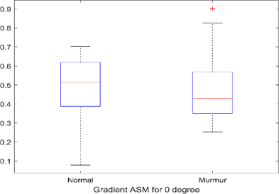
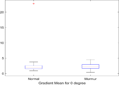
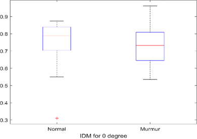
Figures 6 to 10 show the calculated GLDM properties at distance d = 1 and angle 0°. In general, it is shown that the resulting characteristics overlap each other. Thus, it can be predicted that the maximum accuracy will not reach 100%. After seeing the distribution of the features obtained, the next step is testing the accuracy using a combination of all the features and characteristics for each GLDM angle.
Figure 6. Boxplot of gradient contrast for 0°
Figure 7. Boxplot of gradient ASM for 0°
Figure 8. Boxplot of gradient entropy for 0°
Figure 9. Boxplot of gradient mean for 0°
Figure 10. Boxplot of IDM for 0°
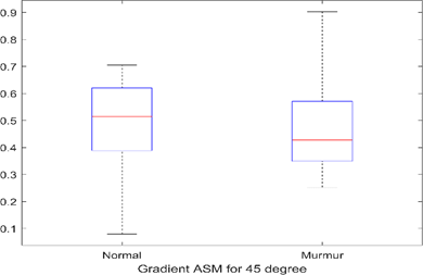
Figure 11. Boxplot of gradient contrast for 45°
Figure 12. Boxplot of gradient ASM for 45°
Figure 13. Boxplot of gradient entropy for 45°
Figure 14. Boxplot of gradient mean for 45°
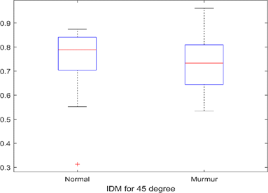
Figure 15. Boxplot of IDM for 45°
Figure 16. Boxplot of gradient contrast for 90°
Figure 17. Boxplot of gradient ASM for 90°
Figure 18. Boxplot of gradient entropy for 90°
Figure 19. Boxplot of gradient mean for 90°
Figure 20. Boxplot of IDM for 90°
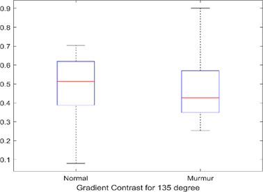
Figure 21. Boxplot of gradient contrast for 135°
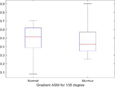
Figure 22. Boxplot of gradient ASM for 135°
Figure 23. Boxplot of gradient entropy for 135°
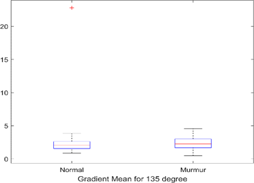
Figure 24. Boxplot of gradient mean for 135°
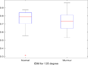
Figure 25. Boxplot of IDM for 135°
Figures 11 – 25 show the 5 GLDM features for angles of 45°, 90°, and 135° for intuitive comparison. In general, the characteristics of the two types of heart sounds overlap. This will affect the accuracy to be achieved. Using one feature will not produce high accuracy, so a combination of several features is needed.
The accuracy obtained by using 3-fold CV, and 5-fold CV is shown in Table 1 and Table 2. Table 1 and Table 2 show the accuracy under STFT conditions using three parameters, three types of SVM kernel, and GLDM angle. The highest accuracy reaches 83% using STFT 200-100 on linear SVM utilizing a combination of GLDM features. Meanwhile, the highest accuracy in using features in one direction only reaches 74% using an angle of 135°, with a resolution of 200-100 STFT and Cubic SVM. It is generally seen that the STFT resolution of 200-100 tends to produce higher accuracy. The STFT 200-100 provides moderate resolution compared to the 500-475 and 25-20. Differences in parameter determination on STFT will result in different resolutions. As we know, the resolution of the STFT is determined by the NFFT and the windowing width used. This will affect the texture of the resulting image.
Table 1. Accuracy (%) using 3-fold cross-validation
|
GLDM features |
Spectrogram parameters |
SVM Kernels |
||
|
Linear |
Quadratic |
Cubic |
||
|
Composite |
500-475 |
71 |
75 |
69 |
|
200-100 |
78 |
75 |
74 |
|
|
25-20 |
74 |
74 |
80 |
|
|
0° |
500-475 |
62 |
65 |
58 |
|
200-100 |
63 |
65 |
73 |
|
|
25-20 |
70 |
67 |
66 |
|
|
45° |
500-475 |
66 |
69 |
55 |
|
200-100 |
63 |
67 |
68 |
|
|
25-20 |
68 |
68 |
69 |
|
|
90° |
500-475 |
67 |
70 |
64 |
|
200-100 |
64 |
64 |
61 |
|
|
25-20 |
65 |
59 |
53 |
|
|
135° |
500-475 |
68 |
72 |
61 |
|
200-100 |
63 |
69 |
72 |
|
|
25-20 |
69 |
68 |
69 |
|
Table 2. Accuracy (%) using 5-fold cross-validation
|
GLDM features |
Spectrogram parameters |
SVM Kernels |
||
|
Linear |
Quadratic |
Cubic |
||
|
Composite |
500-475 |
72 |
76 |
79 |
|
200-100 |
83 |
80 |
82 |
|
|
25-20 |
66 |
77 |
77 |
|
|
0° |
500-475 |
69 |
69 |
56 |
|
200-100 |
69 |
66 |
72 |
|
|
25-20 |
68 |
69 |
68 |
|
|
45° |
500-475 |
67 |
62 |
63 |
|
200-100 |
70 |
67 |
73 |
|
|
25-20 |
68 |
66 |
64 |
|
|
90° |
500-475 |
65 |
72 |
63 |
|
200-100 |
64 |
69 |
59 |
|
|
25-20 |
65 |
60 |
50 |
|
|
135° |
500-475 |
68 |
66 |
61 |
|
200-100 |
65 |
64 |
74 |
|
|
25-20 |
69 |
67 |
70 |
|
In this study, GLDM features are used for feature extraction from the converted image from STFT. This method is different from the previous studies that carried out direct feature calculations on STFT [21]. In the case of direct feature calculations from STFT, statistical parameters used usually such as mean, variance, entropy, skewness, and kurtosis. As shown in Table 3 that shows the accuracy of the STFT statistical characteristics, which results in a maximum accuracy of 72% on the STFT 512-25-20 and 5fold CV.
Table 3. Accuracy (%) using statistical parameter on STFT and 5-fold cross-validation
|
Spectrogram parameters |
SVM Kernels |
||
|
Linear |
Quadratic |
Cubic |
|
|
500-475 |
60 |
54 |
51 |
|
200-100 |
70 |
68 |
63 |
|
25-20 |
72 |
69 |
57 |
Compared with previous studies using fractal dimensions, the accuracy in this study is relatively lower [16]. The fractal method yielded an accuracy of 86.67% [16]. In this research, the PCG signal is filtered, then the wavelet decomposes, and then Fourier transform is performed to obtain the signal's frequency spectrum. Higuchi fractal dimension (HFD) was calculated signal spectrum with various Kmax values. In this study, the characteristics were taken in the frequency domain, while in our proposed method, heart sound in the time-frequency domain was converted into a spatial domain. The proposed method has the advantage of viewing signals in the time-frequency domain, which means that more information can be obtained from heart sound signals.
The proposed method uses a combination of STFT and GLDM for feature extraction to classify heart sounds. STFT displays the signal in the time-frequency domain. The signal distribution in the time and frequency domains is quantized using GLDM. With this method, the information in the heart sounds obtained is more comprehensive. Another advantage of this method is that the number of features produced does not depend on the length of the signal, namely five features multiplied by the number of angles to be calculated. Although the STFT size depends on the signal length, segmentation process, windowing, and N-FFT, the GLDM process produces a fixed number of features. This research still can be further developed, such as exploring the appropriate STFT resolution and other image analysis methods. The use of GLDM for selecting the optimal pixel distance is also interesting [22].
This study has demonstrated a novel method to classify the normal heart sounds and murmurs based on image analyses using GLDM. STFT is performed on heart sounds to obtain a spectrogram of heart sounds. The spectrogram is treated as an image after going through the conversion process. GLDM characteristics are calculated at angles of 0°, 45°, 90°, and 135°. SVM is used as a classifier with three kinds of kernels. The highest accuracy is achieved using STFT with a window width of 200-100 and a combination of all the features of GLDM. GLDM only produces the highest accuracy of 73% using features in one direction. This is due to the characteristic resulting in the relative overlap between normal heart sounds and murmurs. The results obtained provide an opportunity further to explore the use of image analysis on 1D signals. The use of signal transformation methods to other TF domains is one form of development in further research and other image analysis methods.
This work was financially supported by Telkom University, Indonesia.
[1] Ismail, S., Siddiqi, I., Akram, U. (2018). Localization and classification of heart beats in phonocardiography signals—A comprehensive review. EURASIP Journal on Advances in Signal Processing, 2018(1): 1-27. https://doi.org/10.1186/s13634-018-0545-9
[2] Szymanowska, O., Zagrodny, B., Ludwicki, M., Awrejcewicz, J. (2016). Development of an Electronic Stethoscope. Mechatronics: Ideas, Challenges, Solutions and Applications. Cham: Springer International Publishing, 189-204. http://dx.doi.org/10.1007/978-3-319-26886-6_12
[3] Li, F., Liu, M., Zhao, Y., Kong, L., Dong, L., Liu, X., Hui, M. (2019). Feature extraction and classification of heart sound using 1D convolutional neural networks. EURASIP Journal on Advances in Signal Processing, 2019(1): 1-11. https://doi.org/10.1186/s13634-019-0651-3
[4] Hamidi, M., Ghassemian, H., Imani, M. (2018). Classification of heart sound signal using curve fitting and fractal dimension. Biomedical Signal Processing and Control, 39: 351-359. http://dx.doi.org/10.1016/j.bspc.2017 .08.002
[5] Li, S., Li, F., Tang, S., Xiong, W. (2020). A review of computer-aided heart sound detection techniques. BioMed Research International, 2020: 5193707. https://doi.org/10.1155/2020/5846191
[6] Hadiyoso, S., Rizal, A. (2021). Empirical mode decomposition and grey level difference for lung sound classification. Traitement du Signal, 38(1): 175-179. http://dx.doi.org/10.18280/ts.380118
[7] Padilla-Ortiz, A.L., Ibarra, D. (2018). Lung and heart sounds analysis: state-of-the-art and future trends. Critical Reviews™ in Biomedical Engineering, 46(1): 33-52. http://dx.doi.org/10.1615/CritRevBiomedEng.2018025112
[8] Wang, Y., Li, W., Zhou, J., Li, X., Pu, Y. (2014). Identification of the normal and abnormal heart sounds using wavelet-time entropy features based on OMS-WPD. Future Generation Computer Systems, 37: 488-495. http://dx.doi.org/10.1016/j.future.2014.02.009
[9] Komalasari, R., Rizal, A., Suratman, F.Y. (2020). Classification of normal and murmur hearts sound using the fractal method. International Journal, 9(5): 8178-8183. http://dx.doi.org/10.30534/ijatcse/2020/181952020
[10] Zhang, W., Han, J., Deng, S. (2017). Heart sound classification based on scaled spectrogram and tensor decomposition. Expert Systems with Applications, 84: 220-231. https://doi.org/10.1016/j.eswa.2017.05.014
[11] Langley, P., Murray, A. (2017). Heart sound classification from unsegmented phonocardiograms. Physiological Measurement, 38(8): 1658. https://doi.org/10.1088/ 1361-6579/aa724c
[12] Rizal, A., Priharti, W., Hadiyoso, S. (2021). Seizure detection in Epileptic EEG using short-time Fourier transform and support vector machine. International Journal of Online & Biomedical Engineering, 17(14): 65-78. http://dx.doi.org/10.3991/ijoe.v17i14.25889
[13] Weszka, J.S., Dyer, C.R., Rosenfeld, A. (1976). A comparative study of texture measures for terrain classification. IEEE transactions on Systems, Man, and Cybernetics, 4: 269-285. https://doi.org/10.1109/TSMC.1976.5408777
[14] Das, D., Mahanta, L.B., Ahmed, S., Baishya, B.K., Haque, I. (2019). Automated classification of childhood brain tumours based on texture feature. Songklanakarin Journal of Science & Technology, 41(5): 1014-1020. http://dx.doi.org/10.14456/sjst-psu.2019.128
[15] Kalyan, K., Jakhia, B., Lele, R.D., Joshi, M., Chowdhary, A. (2014). Artificial neural network application in the diagnosis of disease conditions with liver ultrasound images. Advances in Bioinformatics, 2014: 708279. https://doi.org/10.1155/2014/708279
[16] Juniati, D., Khotimah, C., Wardani, D.E.K., Budayasa, K. (2018). Fractal dimension to classify the heart sound recordings with KNN and fuzzy c-mean clustering methods. In Journal of Physics: Conference Series, 953(1): 012202. https://doi.org/10.1088/1742-6596/953/1/012202
[17] Goldberger, A.L., Amaral, L.A., Glass, L., et al. (2000). PhysioBank, PhysioToolkit, and PhysioNet: Components of a new research resource for complex physiologic signals. Circulation, 101(23): e215-e220. https://doi.org/10.1161/01.CIR.101.23.e215
[18] Liu, C., Springer, D., Li, Q., et al. (2016). An open access database for the evaluation of heart sound algorithms. Physiological Measurement, 37(12): 2181. https://doi.org/10.1088/0967-3334/37/12/2181
[19] Manhertz, G., Bereczky, A. (2021). STFT spectrogram based hybrid evaluation method for rotating machine transient vibration analysis. Mechanical Systems and Signal Processing, 154: 107583. https://doi.org/10.1016/j.ymssp.2020. 107583
[20] Rizal, A., Priharti, W., Rahmawati, D., Mukhtar, H. (2022). Classification of pulmonary crackle and normal lung sound using spectrogram and support vector machine. In Journal of Biomimetics, Biomaterials and Biomedical Engineering, 55: 143-153. https://doi.org/10.4028/p-tf63b7
[21] Rizal, A., Hidayat, R., Nugroho, H.A. (2016). Lung sounds classification using spectrogram's first order statistics features. In 2016 6th International Annual Engineering Seminar (InAES), Yogyakarta, Indonesia, pp. 96-100. https://doi.org/10.1109/INAES.2016.7821914
[22] Rao, K.R., Naganjaneyulu, S. (2021). Permissioned healthcare blockchain system for securing the EHRs with privacy preservation. Ingénierie des Systèmes d’Information, 26(4): 393-402. https://doi.org/10.18280/isi.260407