Maysoon A. Jamal*| Ihab A. El-Khodary | Doaa S. Ali
© 2022 IIETA. This article is published by IIETA and is licensed under the CC BY 4.0 license (http://creativecommons.org/licenses/by/4.0/).
OPEN ACCESS
The measure of efficiency for the supply chain is necessary to show productivity and how it uses its resources. One of the most important efficiency measurements is Data Envelopment Analysis (DEA). The traditional DEA model treats the decision-making units (DMUs) as a black box. It considers only the initial inputs and the final outputs. But the internal interactions between subsystems are neglected. This type of DEA is used for straightforward systems, but the complex multistage systems like supply chains, traditional DEA get inaccurate efficiency indicators. As well as, one of the main challenges is the uncertainty of data. The inputs and outputs values are usually required to be deterministic in traditional DEA. Although, this is not a case of real-life problems. Therefore, we develop a mixed innovative approach from Two-stage DEA and rough set theory to produce a modified Two-stage RDEA. The proposed model can measure the efficiency of DMUs comprehensively by considering the internal structure of any supply chain and treating with incomplete and imprecise data. We applied the Two-stage RDEA model in a three-level supply chain to show its applicability to measure the efficiency for both a whole supply chain and all levels comprehensively.
data envelopment analysis, decision-making units, rough set theory, two-stage RDEA
In the era of globalization, supply chain management (SCM) plays an important role in the business administration field due to the increase in the number of competitors in market globalization. At the beginning of the 1990s, SCM appeared and was concerned with the planning of supply and demand, managing the production and manufacturing, controlling the inventory level, and distributing the products. Performance evaluation is the ability of a firm to produce maximum outputs by using a set of available inputs. The firm is efficient if it achieves maximum output with a set of inputs [1]. The measure of efficiency is depended on the objective of the government, e.g., minimizing the use of resources (input-oriented), minimizing cost, maximizing productivity (output-oriented), or maximizing profit. from this perspective, supply chain efficiency is how the firm utilizes the resources to achieve its goal in the whole supply chain and it’s all levels.
Data Envelopment Analysis is one of the most popular methods in performance efficiency evaluation. DEA is a data-oriented approach. It is a nonparametric mathematical-based tool that transforms multiple inputs into multiple outputs to evaluate the efficiency and performance of a set of entities DMUs. The result from the DEA study is classified all DMUs as either “efficient” or “inefficient”. Efficiency is defined simply as a ratio when the case has a single input and output. However, in real-life, any organization have multiple inputs and output. The efficiency of a DMU is measured relative to all other DMUs. Each DMU is calculated and analyzed to get the maximum performance for each unit separately.
Chames, Cooper, and Rhodes, (CCR model) [2] consider the fundamental DEA model, built to measure the efficiency of DMUs. The obtained efficiency is not absolute efficiency but relative efficiency to other DMUs which are measured. CCR model is considered the birth of DEA and is still the most widely used type of DEA model. After that, Banker, Charnes, & Cooper 1984 [3] developed the BCC model which is VRS. It uses only when required to check for increasing or decreasing returns because its interpretations for results are complicated. On the contrary, the CCR model is most commonly used because it is easy and better in interpreting results. Recently, the DEA models are becoming popular for evaluating the relative efficiency in different sectors (e.g., education, healthcare, economy, etc.). It determines the efficiency based on its inputs and outputs and compares it with the other DMUs involved in the analysis.
In the traditional DEA, the supply chain is treated as a black box where the initial inputs from the first stage and the final outputs from the last stage only are considered. That is, all the intermediate stages are neglected which makes the efficiency evaluation not accurate and the results may not make sense. Therefore, the evaluation in the form of a network (i.e. evaluate the DMUs in multi-stages not evaluate all the processes as one stage, by considering only the initial inputs and final outputs) is considered a good solution for solving this problem.
A two-stage DEA model was developed to measure the internal efficiency of any sub-systems [4]. The traditional DEA model was modified to can measure the efficiency of the series relationship of the two sub-processes within the whole process. In Two-stage DEA models, the first stage consumes some inputs and produces some outputs. The outputs of the first stage are used as the inputs of the second stage. These are called the intermediate variables.
The anther limitation in applying traditional DEA to measure the efficiency of a supply chain is uncertainty. In the traditional DEA, all variables are required to be deterministic, and this is not the case in most real-life problems. Unfortunately, the most of observed data are vague, imprecise, and incomplete. Usually, data is vague like the production amount. Most of the time there is no exact amount of products produced, but it depends on estimations. In addition, data may be imprecise like time, cost of production, and cost of transportation. That makes the efficiency evaluation process results inaccurate and does not represent reality. After stochastic DEA and fuzzy DEA. Rough DEA is a new tool used to deal with uncertainty. So in our study, To overcome this problem. we use Rough DEA to can treat the rough uncertain environment in the supply chain.
In this paper, we integrate two-stage DEA and rough set theory to produce a two-stage RDEA model that overcomes the most two popular problems faced by decision-makers in the efficiency evaluation of any system. That is the Uncertainty and vague data, and the multi-stage systems with dependent relations like supply chains. In the previous studies, the two-stage DEA and rough DEA are used separately. This paper aims to develop a model that can open the black box and evaluate the complex systems (e.g. supply chain) with internal relations between its stages. As well as, can be treated with vague, uncertain, imprecise data for inputs and outputs values. In the two-stage RDEA, we use the α-optimistic and α-pessimistic method which transforms rough variables into a deterministic form which is necessary for the DEA method. After that, we use Wang and chin [5] method to transform two-stage into one stage to evaluate the efficiency of the whole system and all its subsystem comprehensively. Our proposed model will apply to a three-level supply chain of a cement company to show its ability to treat with multi-stage supply chain with rough inputs and outputs variables.
The rest of the paper is represented as follows: section 2. shows a background about two-stage DEA and rough DEA. In section 3, we introduce the proposed model (i.e., Two-stage RDEA) in detail and show how merging Two-stage DEA and rough set theory to produce our proposed model. In section 4, we apply our proposed model on a three-level supply chain example to evaluate the efficiency of the whole supply chain and its two stages. Finally, section 5 concludes the work and discusses future works.
2.1 Rough data envelopment analysis (RDEA)
As mentioned before the inputs and outputs values in the traditional measuring efficiency methods like DEA are usually required exact values. Although, the supply chains usually have uncertain inputs and outputs. The most of time, the data observed are ambiguous, not precise, or taken at a specific point in time, which considers an inaccurate representation of the distribution of all the data.
The rough set theory is a new mathematical tool that was introduced by Pawlak [6]. After stochastic theory and fuzzy set theory [7]. While Liu [8] proposed rough variables for dealing with vague, imprecise, and uncertain data. As a general assumption, any object is described by information and in real life, this information may not be enough to describe it exactly so it can be approximated by sets. The lower and upper sets are used to define the rough variables (X̱,X̅). A rough variable ξ is represented by four parameters ([a,b],[c,d]) where c≤a<b≤d.In this study, we use the α-optimistic and α-pessimistic method to convert the rough variables to deterministic variables. Suppose there are n DMUs (supply chains) each DMU has x inputs and y outputs. The CCR DEA is represented by:
$Z_{0}=\operatorname{Max} \sum_{r=1}^{s} y_{r 0} u_{r}$
s.t. $\sum_{i=1}^{m} x_{i 0} v_{i}=1$
$\sum_{r=1}^{s} y_{r j} u_{r}-\sum_{i=1}^{m} x_{i j} v_{i} \leq 0(j=1,2,3, \ldots, n)$
$u_{r}, v_{i} \geq 0$ (1)
where, i=1, 2, 3, …, m; r=1, 2, 3, …, s.
The DEA with rough inputs values (x̂) and rough outputs values ($\hat{y}$) transform Eq. (1) to:
$Z_{0}=\operatorname{Max} \sum_{r=1}^{s} \hat{y}_{r 0} u_{r}$
s.t. $\sum_{i=1}^{m} \hat{x}_{i 0}=1$
$\sum_{r=1}^{s} \hat{y}_{r j} u_{r}-\sum_{i=1}^{m} \hat{x}_{i j} v_{i} \leq 0 \quad(j=1,2,3, \ldots, n)$
$v_{i}, u_{r} \geq 0$ (2)
where, i=1, 2, 3, …, m; r=1, 2, 3, …, s.
A rough variable ξ has an α-optimistic value and α-pessimistic value, upper bound and lower bound, respectively. They are donated as:
$\xi_{s u p}(\alpha)=\left\{\begin{array}{c}(1-2 \alpha) d+2 \alpha c, \alpha \leq\left(\frac{d-b}{[2(d-c)]}\right) \\ 2(1-\alpha) d+(2 \alpha-1) c, \alpha \geq\left(\frac{2 d-a-c}{[2(d-c])}\right) \\ \frac{d(b-a)+b(d-c)-2 \alpha(b-a)(d-c)}{(b-a)+(d-c)}, \text { otherwise }\end{array}\right.$ (3)
$\xi_{\text {inf }}(\alpha)=\left\{\begin{array}{c}(1-2 \alpha) c+2 \alpha d, \alpha \leq\left(\frac{a-c}{[2(d-c)]}\right) \\ 2(1-\alpha) c+(2 \alpha-1) d, \alpha \geq\left(\frac{b+d-2 c}{[2(d-c])}\right) \\ \frac{c(b-a)+a(d-c)+2 \alpha(b-a)(d-c)}{(b-a)+(d-c)}, \text { otherwise }\end{array}\right.$ (4)
For a rough variable ξ:
2.2 Two-stage data envelopment analysis (Two-stage DEA)
The main limitation of the traditional DEA model is the “black box” theory. It reflects inaccurate efficiency indicators about the supply chains which consist of complex structures. Because it treats the production process like a black box, in which the input variables are transformed within this box to give the output variables. The traditional DEA model has only input and output variables and based on the relationship between these variables, the DEA indicates which DMUs are efficient.
Therefore, recently many studies [9-11] have focused on the Two-stage DEA model, which allows to open the box and go internally. And divide the production process into subprocesses. each subprocess has its inputs and outputs. the efficiency evaluation in Two-stage DEA contains two steps. The first step, evaluate each subprocess separately. The second step, evaluate the whole process. Wherefore, Two-stage DEA gets a comprehensive efficiency and helps the decision-makers to know which subprocess is inefficient and improves the efficiency of the whole system.
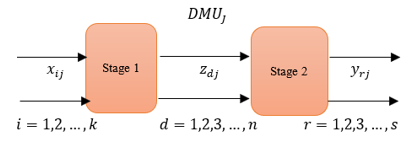
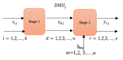
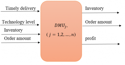
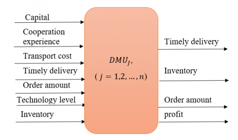
In real-life, subsystems are connected as a network. There are two types of network structure. Type I (basic network) [9] consider the outputs from the first stage will be the only inputs for the second stage without external inputs entering in the intermediate stage as shown in Figure 1. Basic two-stage DEA is the simplest form for two-stage DEA. Type II (general network) [4] allowed external inputs to enter the second stage in addition to the outputs from the first stage Figure 2.
In basic two-stage DEA (Figure 1) we can notice that for every DMUj there are a number of inputs xij entered to stage 1 and produce a number of outputs zdj. The outputs zdj from stage 1 enter to stage 2 as inputs this called intermediate values, then the intermediate values produce final outputs ydj from stage 2. But in general, in two-stage DEA, (Figure 2) there is an additional external input hmj (e.g.,” Technology level” in the practical example below) enter to stage 2.
Seiford et al. [12] used a two-stage DEA model for 55 commercial banks that contain the profitability and marketability as two separated stages and tried to measure the efficiency for each stage. In this model there is no serial relation between the two stages, the sub-processes are complete independently.
Kao and Hwang [9] measured the efficiency of 24 non-life insurance companies in Taiwan by using constant return to scale (CRS) two-stage DEA, they modified the model [12] to contain a relation between the subprocesses by making the output from stage 1 is input for stage 2.
In (2010) Wang and Chin [5] developed a model by adding relative weights for the two stages of processes to can treated with a CRS and a variable return to scale (VRS) models. In this paper, we use Wang and Chin model. The model of Wang and Chin assigned two weights λ1≥0 and λ2≥0, where λ1+λ2=1 to Kao and Hwang’s model to be general and can use to calculate the efficiency of CRS and VRS models. Therefore, to get the efficiency for every DMUJ, in stage 1 and stage 2 respectively will be:
$\theta_{j}^{1 *}=\sum_{d=1}^{D} \eta_{d}^{1} z_{d j} / \sum_{i=1}^{m} v_{i} x_{i j}, \theta_{j}^{2 *}=\sum_{r=1}^{s} u_{r} y_{r j} / \sum_{d=1}^{D} \eta_{d}^{2} z_{d j}$
where,
The total efficiency for the two-stage DEA model is defined by:
$\theta_{0}^{*}=\lambda_{1} \theta_{0}^{1 *}+\lambda_{2} \theta_{0}^{2 *}$
$\theta_{0}^{*}=\operatorname{Max} \lambda_{1} \sum_{d=1}^{D} \eta_{d} z_{d 0}+\lambda_{2} \sum_{r=1}^{s} u_{r} y_{r 0}$
s.t $\lambda_{1} \sum_{i=1}^{m} v_{i} x_{i 0}+\lambda_{2} \sum_{d=1}^{D} \eta_{d} z_{d 0}=1$
$\sum_{d=1}^{D} \eta_{d} z_{d j}-\sum_{i=1}^{m} v_{i} x_{i j} \leq 0(j=1,2,3, \ldots, n)$
$\sum_{r=1}^{s} u_{r} y_{r j}-\sum_{d=1}^{D} \eta_{d} z_{d j} \leq 0(j=1,2,3, \ldots, n)$
$v_{i}, \eta_{d}, u_{r} \geq 0$ (5)
where, i=1, 2, 3, …, m, d=1, 2, 3, …, D, r=1, 2, 3, …, s.
Figure 1. A basic structure for the two-stage DEA
Figure 2. A general structure for two-stage DEA
3.1 The combination of two-stage DEA and rough set theory
In the section, we show how can merge two-stage DEA and rough set theory. The combined model can use to solve the problem of black-box efficiency evaluation and uncertain data in inputs and outputs. By evaluating the whole system and its subsystems with considering vague and incomplete data.
A two-stage RDEA consists of merging Eq. (2) and Eq. (5) to produce:
$\theta_{0}^{*}=\operatorname{Max}_{1} \sum_{d=1}^{D} \eta_{d} \hat{\mathrm{z}}_{d 0}+\lambda_{2} \sum_{r=1}^{s} u_{r} \hat{\mathrm{y}}_{r 0}$
s.t.
$\lambda_{1} \sum_{i=1}^{m} v_{i} \hat{x}_{i 0}+\lambda_{2} \sum_{d=1}^{D} \eta_{d} \hat{\mathrm{z}}_{d 0}=1$
$\sum_{d=1}^{D} \eta_{d} \hat{\mathrm{z}}_{d j}-\sum_{i=1}^{m} v_{i} \hat{x}_{i j} \leq 0(j=1,2,3, \ldots, n)$
$\sum_{r=1}^{s} u_{r} \hat{\mathrm{y}}_{r j}-\sum_{d=1}^{D} \eta_{d} \hat{z}_{d j} \leq 0(j=1,2,3, \ldots, n)$
$v_{i}, \eta_{d}, u_{r} \geq 0$ (6)
where, i=1, 2, 3, …, m; d=1, 2, 3, …, D; r=1, 2, 3, …, s.
We use the α-optimistic and α-pessimistic method to convert the rough variables $\hat{X} j, \hat{Y} j, \hat{Z} j$ to deterministic variables, this is done through two steps.
In the first step, where 0.5˂α≤1, then $\theta_{0}^{\inf (\alpha)} \geq \theta_{0}^{\sup (\alpha)}$. Therefore, Eq. (6) will convert to an interval programming model:
$\theta_{0}^{*}=M a x \lambda_{1} \sum_{d=1}^{D} \eta_{d}\left[Z_{d 0}^{\sup (\alpha)}, Z_{d 0}^{\inf (\alpha)}\right]$
$+\lambda_{2} \sum_{r=1}^{s} u_{r}\left[Y_{r 0}^{\sup (\alpha)}, Y_{r 0}^{\inf (\alpha)}\right]$
s.t. $\lambda_{1} \sum_{i=1}^{m} v_{i}\left[X_{i 0}^{\sup (\alpha)}, X_{i 0}^{\inf (\alpha)}\right]+\lambda_{2} \sum_{d=1}^{m} \eta_{d}\left[Z_{d 0}^{\sup (\alpha)}, Z_{d 0}^{\inf (\alpha)}\right]=1$
$\sum_{d=1}^{D} \eta_{d}\left[Z_{d j}^{\sup (\alpha)}, Z_{d j}^{\inf (\alpha)}\right]-\sum_{i=1}^{m} v_{i}\left[X_{i j}^{\sup (\alpha)}, X_{i j}^{\inf (\alpha)}\right] \leq 0$
$\sum_{r=1}^{s} u_{r}\left[Y_{r j}^{\sup (\alpha)}, Y_{r j}^{\inf (\alpha)}\right]-\sum_{d=1}^{D} \eta_{d}\left[Z_{d j}^{\sup (\alpha)}, Z_{d j}^{\inf (\alpha)}\right] \leq 0$
$v_{i}, \eta_{d}, u_{r} \geq 0$ (7)
where, i=1, 2, 3, …, m; d=1, 2, 3, …, D; r=1, 2, 3, …, s; j=1, 2, 3, …, n.
The second step, convert the interval programming Eq. (7) to a deterministic linear programming model. Consequently, Eq. (7) divide into two deterministic linear programming to get the lower bound ($\theta_{0}^{\sup (\alpha)}$) and upper bound $\left(\theta_{0}^{\inf (\alpha)}\right)$.
To get the minimum linear programming of Eq. (7) $\left(\theta_{0}^{\sup (\alpha)}\right)$, under trust level $\alpha$. Let DMU0 be the evaluated DMU and will compare it with the rest of the DMUs. In the worst case, the inputs for DMU0 have maximum values and the outputs have the minimum values compared with the other DMUs. Consequently, the lower bound $\theta_{0}^{\sup (\alpha)}$ donated as:
$\theta_{0}^{\sup (\alpha)}=\operatorname{Max}_{1} \sum_{d=1}^{D} \eta_{d} Z_{d 0}^{\sup (\alpha)}+\lambda_{2} \sum_{r=1}^{s} u_{r} Y_{r 0}^{\sup (\alpha)}$
s.t. $\lambda_{1} \sum_{i=1}^{m} v_{i} X_{i 0}^{\inf (\alpha)}+\lambda_{2} \sum_{d=1}^{D} \eta_{d} Z_{d 0}^{\inf (\alpha)}=1$
$\sum_{d=1}^{D} \eta_{d} Z_{d 0}^{\sup (\alpha)}-\sum_{i=1}^{m} v_{i} X_{i 0}^{\inf (\alpha)} \leq 0(j=0)$
$\sum_{d=1}^{D} \eta_{d} Z_{d j}^{\inf (\alpha)}-\sum_{i=1}^{m} v_{i} X_{i j}^{\sup (\alpha)} \leq 0(j=1,2,3, \ldots, n)$
$\sum_{r=r f 1}^{s} u_{r} Y_{r 0}^{\sup (\alpha)}-\sum_{d=1}^{D} \eta_{d} Z_{d 0}^{\inf (\alpha)} \leq 0(j=0)$
$\sum_{r=1}^{s} u_{r} Y_{r j}^{\inf (\alpha)}-\sum_{d=1}^{D} \eta_{d} Z_{d j}^{\sup (\alpha)} \leq 0(j=1,2,3, \ldots, n)$
$v_{i}, \eta_{d}, u_{r} \geq 0$ (8)
where, i=1, 2, 3, …, m; d=1, 2, 3, …, D; r=1, 2, 3, …, s.
Furthermore, to get the maximum linear programming of Eq. (7) $\left(\theta_{0}^{\inf (\alpha)}\right)$, under trust level $\alpha$. Let DMU0 be the evaluated DMU and will compare it with the rest of the DMUs. In the best case, the inputs for DMU0 have minimum values and the outputs have the maximum values compared with the other DMUs. Consequently, the upper bound $\theta_{0}^{\inf (\alpha)}$ donated as:
$\theta_{0}^{\inf (\alpha)}=\operatorname{Max} \lambda_{1} \sum_{d=1}^{D} \eta_{d} Z_{d 0}^{\inf (\alpha)}+\lambda_{2} \sum_{r=1}^{s} u_{r} Y_{r 0}^{\inf (\alpha)}$
s.t. $\lambda_{1} \sum_{i=1}^{m} v_{i} X_{i 0}^{\sup (\alpha)}+\lambda_{2} \sum_{d=1}^{D} \eta_{d} Z_{d 0}^{\sup (\alpha)}=1$
$\sum_{d=1}^{D} \eta_{d} Z_{d 0}^{\inf (\alpha)}-\sum_{i=1}^{m} v_{i} X_{i 0}^{\sup (\alpha)} \leq 0(j=0)$
$\sum_{d=1}^{D} \eta_{d} Z_{d j}^{\sup (\alpha)}-\sum_{i=1}^{m} v_{i} X_{i j}^{\inf (\alpha)} \leq 0(j=1,2,3, \ldots, n)$
$\sum_{r=1}^{s} u_{r} Y_{r 0}^{\inf (\alpha)}-\sum_{d=1}^{D} \eta_{d} Z_{d 0}^{\sup (\alpha)} \leq 0(j=0)$
$\sum_{r=1}^{s} u_{r} Y_{r j}^{\sup (\alpha)}-\sum_{d=1}^{D} \eta_{d} Z_{d j}^{\inf (\alpha)} \leq 0(j=1,2,3, \ldots, n)$
$v_{i}, \eta_{d}, u_{r} \geq 0$ (9)
where, i=1, 2, 3, …, m; d=1, 2, 3, …, D; r=1, 2, 3, …, s.
From solving linear programming (8) and (9), we obtain the relative efficiency interval [θsup(α),θinf(α)] for DMU0 compared with the n-1 DMUs.
3.2 A modified two-stage RDEA in measuring the efficiency for three-level supply chains
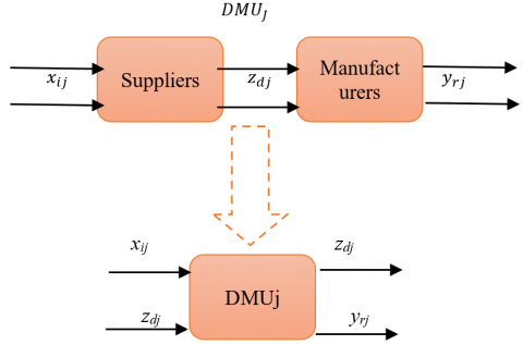
This study aims to apply our proposed model that can use to get a comprehensive efficiency for the entire supply chain which contains multi-level subchains. We apply our model in three-level supply chains that contain suppliers, manufacturers, and distributors as shown in Figure 3.
Figure 3. Three-level supply chain
In the previous section, we discuss how to measure the efficiency of a supply chain that contains two stages and has some rough variables. Here, we introduce how we generalize model (6) to measure the efficiency of multi-level supply chains comprehensively with rough variables. The modified model will be as:
$\theta_{0}^{*}=\operatorname{Max} \lambda_{1}\left(\sum_{d=1}^{D} \eta_{d} \hat{\mathrm{z}}_{d 0}+\sum_{r=1}^{s} u_{r} \hat{\mathrm{y}}_{r 0}\right)$
$+\lambda_{2}\left(\sum_{r=1}^{s} u_{r} \hat{\mathrm{y}}_{r 0}+\sum_{t=1}^{T} \alpha_{t} \hat{w}_{t 0}\right)$
s. t. $\lambda_{1}\left(\sum_{i=1}^{m} v_{i} \hat{x}_{i 0}+\sum_{d=1}^{D} \eta_{d} \hat{\mathrm{z}}_{d 0}\right)+\lambda_{2}\left(\sum_{d=1}^{D} \eta_{d} \hat{\mathrm{z}}_{d 0}+\sum_{r=1}^{m} u_{r} \hat{\mathrm{y}}_{r 0}\right)$
$\left(\sum_{d=1}^{D} \eta_{d} \hat{\mathrm{z}}_{d j}+\sum_{r=1}^{m} u_{r} \hat{\mathrm{y}}_{r j}\right)-\left(\sum_{d=1}^{D} \eta_{d} \hat{\mathrm{z}}_{d j}+\sum_{i=1}^{m} v_{i} \hat{x}_{i j}\right) \leq 0$
$\left(\sum_{r=1}^{s} u_{r} \hat{\mathrm{y}}_{r j}+\sum_{t=1}^{T} \alpha_{t} \hat{w}_{t j}\right)-\left(\sum_{r=1}^{s} u_{r} \hat{\mathrm{y}}_{r j}+\sum_{d=1}^{D} \eta_{d} \hat{z}_{d j}\right) \leq 0$
$v_{i}, \eta_{d}, u_{r}, \alpha_{t} \geq 0$ (10)
where, i=1, 2, 3, …, m; d=1, 2, 3, …, D; r=1, 2, 3, …, s; t=1, 2, 3, …, T.
Model (10) will transform into an interval programming model:
$\begin{aligned} \theta_{0}^{*}=\operatorname{Max}_{1}\left(\sum_{d=1}^{D} \eta_{d}\left[Z_{d 0}^{\sup (\alpha)}, Z_{d 0}^{\inf (\alpha)}\right]\right.\\ &\left.+\sum_{r=1}^{s} u_{r}\left[Y_{r 0}^{\sup (\alpha)}, Y_{r 0}^{\inf (\alpha)}\right]\right) \\ &+\lambda_{2}\left(\sum_{r=1}^{s} u_{r}\left[Y_{d 0}^{\sup (\alpha)}, Y_{d 0}^{\inf (\alpha)}\right]\right.\\ &\left.+\sum_{t=1}^{T} \alpha_{t}\left[W_{t 0}^{\sup (\alpha)}, W_{t 0}^{\inf (\alpha)}\right]\right) \end{aligned}$
s. t. $\lambda_{1}\left(\sum_{i=1}^{m} v_{i}\left[X_{i 0}^{\sup (\alpha)}, X_{i 0}^{\inf (\alpha)}\right]+\sum_{d=1}^{D} \eta_{d}\left[Z_{d 0}^{\sup (\alpha)}, Z_{d 0}^{\inf (\alpha)}\right]\right)+\lambda_{2}\left(\sum_{d=1}^{D} \eta_{d}\left[Z_{d 0}^{\sup (\alpha)}, Z_{d 0}^{\inf (\alpha)}\right]+\sum_{r=1}^{m} u_{r}\left[Y_{r 0}^{\sup (\alpha)}, Y_{r 0}^{\inf (\alpha)}\right]\right)=1$
$\left(\sum_{d=1}^{D} \eta_{d}\left[Z_{d j}^{\sup (\alpha)}, Z_{d j}^{\inf (\alpha)}\right]+\sum_{r=1}^{m} u_{r}\left[Y_{r j}^{\sup (\alpha)}, Y_{r j}^{\inf (\alpha)}\right]\right)-\left(\sum_{d=1}^{D} \eta_{d}\left[Z_{d j}^{\sup (\alpha)}, Z_{d j}^{\inf (\alpha)}\right]+\sum_{i=1}^{m} v_{i}\left[X_{i j}^{\sup (\alpha)}, X_{i j}^{\inf (\alpha)}\right]\right) \leq 0$
$\left(\sum_{r=1}^{s} u_{r}\left[Y_{r j}^{\sup (\alpha)}, Y_{r j}^{\inf (\alpha)}\right]+\sum_{t=1}^{T} \alpha_{t}\left[W_{t j}^{\sup (\alpha)}, W_{t j}^{\inf (\alpha)}\right]\right)-\left(\sum_{r=1}^{s} u_{r}\left[Y_{r j}^{\sup (\alpha)}, Y_{r j}^{\inf (\alpha)}\right]+\sum_{d=1}^{D} \eta_{d}\left[Z_{d j}^{\sup (\alpha)}, Z_{d j}^{\inf (\alpha)}\right]\right) \leq 0$
$v_{i}, \eta_{d}, u_{r}, \alpha_{t} \geq 0$ (11)
where, i=1, 2, 3, …, m; d=1, 2, 3, …, D; r=1, 2, 3, …, s; t=1, 2, 3, …, T; j=1, 2, 3, …, n.
Model (11) will convert into minimum linear programing and maximum linear programming.
The $\theta_{0}^{\sup (\alpha) *}$ donated as:
$\theta_{0}^{\sup (\alpha)^{*}}=\operatorname{Max} \lambda_{1}\left(\sum_{d=1}^{D} \eta_{d} Z_{d 0}^{\sup (\alpha)}+\sum_{r=1}^{s} u_{r} Y_{r 0}^{\sup (\alpha)}\right)+\lambda_{2}\left(\sum_{r=1}^{s} u_{r} Y_{r 0}^{\sup (\alpha)},+\sum_{t=1}^{T} \alpha_{t} W_{t 0}^{\sup (\alpha)}\right)$
s.t. $\lambda_{1}\left(\sum_{i=1}^{m} v_{i} X_{i 0}^{\inf (\alpha)}+\sum_{d=1}^{D} \eta_{d} Z_{d 0}^{\inf (\alpha)}\right)+\lambda_{2}\left(\sum_{d=1}^{D} \eta_{d} Z_{d 0}^{\inf (\alpha)}+\sum_{r=1}^{m} u_{r} Y_{r 0}^{\inf (\alpha)}\right)=1$
$\left(\sum_{d=1}^{D} \eta_{d} Z_{d 0}^{\sup (\alpha)}+\sum_{r=1}^{m} u_{r} Y_{r 0}^{\sup (\alpha)}\right)-\left(\sum_{d=1}^{D} \eta_{d} Z_{d 0}^{\inf (\alpha)}+\sum_{i=1}^{m} v_{i} X_{i 0}^{\inf (\alpha)}\right) \leq 0(j=0)$
$\left(\sum_{d=1}^{D} \eta_{d} Z_{d j}^{\inf (\alpha)}+\sum_{r=1}^{m} u_{r} Y_{r j}^{\inf (\alpha)}\right)-\left(\sum_{d=1}^{D} \eta_{d} Z_{d j}^{\sup (\alpha)}+\sum_{i=1}^{m} v_{i} X_{i j}^{\sup (\alpha)}\right) \leq 0$
$\left(\sum_{r=1}^{s} u_{r} Y_{r 0}^{\sup (\alpha)}+\sum_{t=1}^{T} \alpha_{t} W_{t 0}^{\sup (\alpha)}\right)-\left(\sum_{r=1}^{s} u_{r} Y_{r 0}^{\inf (\alpha)}+\sum_{d=1}^{D} \eta_{d} Z_{d 0}^{\inf (\alpha)}\right) \leq 0(j=0)$
$\left(\sum_{r=1}^{s} u_{r} Y_{r j}^{\inf (\alpha)}+\sum_{t=1}^{T} \alpha_{t} W_{t j}^{\inf (\alpha)}\right)-\left(\sum_{r=1}^{s} u_{r} Y_{r j}^{\sup (\alpha)}+\sum_{d=1}^{D} \eta_{d} Z_{d j}^{\sup (\alpha)}\right) \leq 0$
$v_{i}, \eta_{d}, u_{r}, \alpha_{t} \geq 0$ (12)
where, i=1, 2, 3, …, m; d=1, 2, 3, …, D; r=1, 2, 3, …, s; t=1, 2, 3, …, T; j=1, 2, 3, …, n.
The $\theta_{0}^{\inf (\alpha) *}$ donated as:
$\theta_{0}^{\inf (\alpha)^{*}}=\operatorname{Max} \lambda_{1}\left(\sum_{d=1}^{D} \eta_{d} Z_{d 0}^{\inf (\alpha)}+\sum_{r=1}^{s} u_{r} Y_{r 0}^{\inf (\alpha)}\right)+\lambda_{2}\left(\sum_{r=1}^{s} u_{r} Y_{r 0}^{\inf (\alpha)},+\sum_{t=1}^{T} \alpha_{t} W_{t 0}^{\inf (\alpha)}\right)$
s.t. $\lambda_{1}\left(\sum_{i=1}^{m} v_{i} X_{i 0}^{\sup (\alpha)}+\sum_{d=1}^{D} \eta_{d} Z_{d 0}^{\sup (\alpha)}\right)+\lambda_{2}\left(\sum_{d=1}^{D} \eta_{d} Z_{d 0}^{\sup (\alpha)}+\sum_{r=1}^{m} u_{r} Y_{r 0}^{\sup (\alpha)}\right)=1$
$\left(\sum_{d=1}^{D} \eta_{d} Z_{d 0}^{\inf (\alpha)}+\sum_{r=1}^{m} u_{r} Y_{r 0}^{\inf (\alpha)}\right)-\left(\sum_{d=1}^{D} \eta_{d} Z_{d 0}^{\sup (\alpha)}+\sum_{i=1}^{m} v_{i} X_{i 0}^{\sup (\alpha)}\right) \leq 0(j=0$
$\left(\sum_{d=1}^{D} \eta_{d} Z_{d j}^{\sup (\alpha)}+\sum_{r=1}^{m} u_{r} Y_{r j}^{\sup (\alpha)}\right)-\left(\sum_{d=1}^{D} \eta_{d} Z_{d j}^{\inf (\alpha)}+\sum_{i=1}^{m} v_{i} X_{i j}^{\inf (\alpha)}\right) \leq 0$
$\left(\sum_{r=1}^{s} u_{r} Y_{t 0}^{\inf (\alpha)}+\sum_{t=1}^{T} \alpha_{t} W_{t 0}^{\inf (\alpha)}\right)-\left(\sum_{r=1}^{s} u_{r} Y_{r 0}^{\sup (\alpha)}+\sum_{d=1}^{D} \eta_{d} Z_{d 0}^{\sup (\alpha)}\right) \leq 0(j=0)$
$\left(\sum_{r=1}^{S} u_{r} Y_{r j}^{\sup (\alpha)}+\sum_{t=1}^{T} \alpha_{t} W_{t j}^{\sup (\alpha)}\right)-\left(\sum_{r=1}^{S} u_{r} Y_{r j}^{\inf (\alpha)}+\sum_{d=1}^{D} \eta_{d} Z_{d j}^{\inf (\alpha)}\right) \leq 0$
$v_{i}, \eta_{d}, u_{r}, \alpha_{t} \geq 0$ (13)
where, i=1, 2, 3, …, m; d=1, 2, 3, …, D; r=1, 2, 3, …, s; t=1, 2, 3, …, T; j=1, 2, 3, …, n.
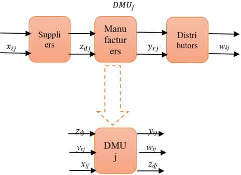
The comprehensive evaluation process for the three-level supply chain in Figure 3 will be summarized in three steps:
First step: split the three-level supply chain into two subchains (suppliers-manufacturers) and (manufacturers- distributors). In this step, we evaluate the efficiency of each subchain separately. Figure 4 and Figure 5 are the transformations for the suppliers-manufacturers subchain and manufacturers-distributors subchain, respectively. Then evaluate each subchain independently by using Eq. (8) and (9), respectively.
Second step: transform the whole three-level supply chain into one stage Figure 6. Then evaluate the whole supply chain by using Eq. (12) and (13).
Based on the results from step one (i.e., efficiency evaluation for each subchain) and step two (i.e., efficiency evaluation for the whole supply chain), we can get a comprehensive efficiency evaluation for each DMUs and determine which DMU is the best.
Third step: is to rank all DMUs (supply chains) according to the MRA method will discuss in the next section.
$\max \left(r_{i}\right)=\max _{j \neq 1}\left\{\theta_{j}^{\inf (\alpha)}\right\}-\theta_{i}^{\sup (\alpha)}$
Figure 4. Two-stage supplier and manufacturer supply chain converted into the one-stage supply chain
Figure 5. Two-stage manufacturer and distributors supply chain converted into the one-stage supply chain
Figure 6. Three-level suppliers, manufacturers, and distributors supply chain converted into the one-stage supply chain
3.3 The ranking method for efficiency DMUs
After we get the efficiency interval for all DMUs, we should rank the efficiency intervals for DMUs. Because in case having more than one DMU is efficient, we can determine which DMU is the most efficient, and order the rest efficient DMUs based on the difference between its upper and lower bound intervals. In this study, we use the MRA approach introduced by Wang et al. [13] to rank the efficient DMUs intervals. In the beginning, we should notice that the three-level supply chain will be efficient only if:
The upper limit $\left(\theta_{0}^{\inf (\alpha) *}\right)$ for all sub-chains=1.
The upper limit $\left(\theta_{0}^{\inf (\alpha) *}\right)$ for the whole supply chain =1.
The MRA approach is introduced as follows:
Compute the maximum loss of efficiency for each efficient DMUs and choose the maximum loss of efficiency (regret).
Compare the regret function for all efficiency intervals and order the DMUs from the minimum regret (no loss of efficiency) to the maximum regret.
$\min _{i}\left\{\max \left(r_{i}\right)\right\}=\min _{i}\left\{\max \left[\max _{j \neq 1}\left(\alpha_{j}^{\inf (\alpha)}\right)-\theta_{i}^{\sup (\alpha)}, 0\right]\right\}$
We apply a two-stage RDEA which is discussed in section 3 on a three-level supply chain for seven cement companies. The three stages of the supply chain are suppliers, manufacturers, and distributors Figure 7. Figures 8-10 show how the whole supply chain and its sub-chains are converted to one stage. Eq. (8) and (9) are used two times to get the efficiency intervals for rough data. First time for the suppliers-manufacturers and the second time for manufacturers- distributors stage. Thereafter, Eq. (12) and (13) are used for a whole supply chain (suppliers-manufacturers-distributors) to compute the efficiency intervals for 7 DMUs. Table 1 shows the inputs and the outputs for suppliers, manufacturers, and distributors (hint: Cooperation Experience is as a qualitative variable, we measure it by years of experience).
Tables 2 and 3 show the values of all inputs and outputs for the seven DMUs.
We discussed before that, in real life the supply chain usually contains uncertain and vague data. In our example, the rough variables are cost, timely delivery, and order amount. To apply two-stage RDEA in a three-level supply chain containing rough variables, we assume that:
There is external input in the manufacturers' stage, so the structure for the two-stage RDEA is a general network.
Figure 7. Three-level supply chain
Table 1. The inputs and outputs for a Three-level supply chain
|
Factors |
Name of index |
Unit of index |
|
suppliers’ inputs |
Capital |
Million dollars |
|
Cooperation experience |
Years |
|
|
Cost |
Hundred thousand dollars |
|
|
suppliers’ outputs/(manufacturers’ inputs) |
Timely delivery |
% |
|
manufacturers’ inputs (external input) |
Technology level |
% |
|
manufacturers’ outputs/distributors’ inputs |
Amount of the order |
1/day |
|
Inventory |
1/day |
|
|
distributors’ outputs |
Profit |
Million dollars |
Table 2. Input variables
|
DMU |
Capital |
Cooperation experience |
Cost |
Timely delivery |
Technology level |
|
1 |
14 |
3 |
(8,9), (6,12) |
(82,85), (80,92) |
86 |
|
2 |
12 |
2 |
(13,14), (11,17) |
(55,58), (53,65) |
75 |
|
3 |
10 |
3 |
(31,32), (28,35) |
(78,81), (76,88) |
73 |
|
4 |
1.6 |
2 |
(14,15), (12,18) |
(67,70), (65,77) |
83 |
|
5 |
10 |
2 |
(24,5), (22,28) |
(61,64), (59,71) |
90 |
|
6 |
7 |
3 |
(51,52), (49,55) |
(70,73), (68,80) |
84 |
|
7 |
3 |
3 |
(36,37), (34,40) |
(74,77), (72,84) |
90 |
Table 3. Output variables
|
DMU |
Timely delivery |
Technology level |
Inventory |
Order amount |
profit |
|
1 |
(82,85), (80,92) |
86 |
53 |
(65,67), (60,72) |
20 |
|
2 |
(55,58), (53,65) |
75 |
74 |
(72,75), (70,83) |
18 |
|
3 |
(78,81), (76,88) |
73 |
82 |
(83,88), (80,95) |
16 |
|
4 |
(67,70), (65,77) |
83 |
62 |
(58,67), (55,70) |
5 |
|
5 |
(61,64), (59,71) |
90 |
79 |
(75,80), (73,85) |
17 |
|
6 |
(70,73), (68,80) |
84 |
90 |
(95,98), (90,100) |
14 |
|
7 |
(74,77), (72,84) |
90 |
55 |
(60,65), (58,70) |
10 |
We solved the numerical example under trust level α=0.9 and λ1=λ2=0.5 in two ways: the traditional DEA model and our proposed model (two-stage RDEA). Table 4 represents the results from applying the traditional DEA (CCR model) in a multi-stage supply chain containing rough variables. Table 5 represents the efficiencies intervals for all DMUs obtained from applying the two-stage RDEA model. We visualize the upper bound (θinf(α)) for all supply chains to be easy to compare between the supply chains and their Figure 11.
Figure 8. Suppliers-manufacturers two stages converted to one-stage
Figure 9. Manufacturers-distributors two-stage converted to one stage
Figure 10. Suppliers-manufacturers- distributors three stages converted to one stage
From the results from Tables 4 and 5, we can notice that:
Now, we use the MRA method to rank the efficient DMUs. But in this example when using two-stage RDEA we can see that DMU3 is the only one that is efficient relative to the rest of the DMUs. Because it's upper bound in the suppliers-manufacturers subchain, manufacturers-distributors subchain, and the whole suppliers-manufacturers-distributors supply chain equal 1. so, there is no need to compute the regret function.
By comparing the results from traditional DEA and our model, we can notice that the traditional DEA rank the DMUs as DMU2>DMU3>DMU5>DMU7>DMU6>DMU4>DMU1, and DMU2 is the efficient DMU relative to the rest of the DMUs. In the reality, DMU3 is the most efficient DMU compared to the seven DMUs.
Table 4. The results from traditional DEA
|
DMU |
Supplier-Manufacturers stage |
Relatively efficient |
|
1 |
0.6023 |
No |
|
2 |
1 |
Yes |
|
3 |
0.9865 |
No |
|
4 |
0.7621 |
No |
|
5 |
0.9530 |
No |
|
6 |
0.8453 |
No |
|
7 |
0.8471 |
No |
Table 5. The result of applying modified two-stage RDEA
|
DMU |
Supplier-Manufacturer stage |
Manufacturer-distributors stage |
Whole supply chain (Supplier-Manufacturer-distributors) |
Relatively efficient |
|
1 |
[0.7271,0.8639] |
[0.7473,0.8406] |
[0.7084,0.8469] |
No |
|
2 |
[0.8898.1] |
[0.7884,1] |
[0.8630,0.9879] |
No |
|
3 |
[1.1] |
[0.8521,1] |
[0.7592,1] |
Yes |
|
4 |
[0.7992,0.9290] |
[0.4947,0.6137] |
[0.6213,0.7519] |
No |
|
5 |
[0.8483,1] |
[0.7300,0.8989] |
[0.7961,0.8109] |
No |
|
6 |
[0.9538,1] |
[0.7068,0.7486] |
[0.67801,0.7539] |
No |
|
7 |
[0.5999,0.7935] |
[0.5332,0.6922] |
[0.5597,0.7320] |
No |
Figure 11. The upper bound θinf(α) under trust level α=0.9
In supply chains, the collected data usually be uncertain and insufficient. As well, most of the supply chains are structured as a network, with dependent relations between its stages. In this network, the outputs from any stage may be the inputs to another stage. The traditional DEA can’t treat the nature of the supply chain, because it requires deterministic data. In addition, DEA treats the supply chain as a black box with considering only the initial inputs and final outputs only and ignoring all internal levels in it. Therefore, we developed a modified two-stage RDEA to deal with uncertain multi-stages supply chains.
The proposed model enables to deal with vague and imprecise data (rough variables). by using α-optimistic and α- pessimistic method to convert this rough data to deterministic data, which is required in DEA. In addition, the Two-stage RDEA opens the black box and evaluates the efficiency for every stage in the supply chain not only the whole supply chain.
The aim of our study is allowing to evaluate multi-level supply chains and their all sub-chains comprehensively, with rough inputs and outputs. In our model, we used the α-optimistic and α-pessimistic method to transform the rough variables into deterministic values to get the efficiency intervals $\left[\theta^{\sup (\alpha)}, \theta^{\inf (\alpha)}\right]$ for all DMUs.After that, ranking the efficient DMUs according to the MRA model.
We verified our model by applying it to a three-level supply chain, From the results, we can show that the modified two-stage RDEA can get a comprehensive efficiency not only for supply chains containing two stages but also for multi-level supply chains. We indicate that the whole supply chain will be efficient if and only if the whole supply chain and all its parts are efficient $\left(\theta^{\inf (\alpha)}=1\right)$.
As future work, the current work can depend on the VRS model instead of the CRS model.
[1] Rogers, E.W., Wright, P.M. (1998). Measuring organizational performance in strategic human resource management: Problems, prospects and performance information markets. Human Resource Management Review, 8(3): 311-331. https://doi.org/10.1016/S1053-4822(98)90007-9
[2] Charnes, A., Cooper, W.W., Rhodes, E. (1978). Measuring the efficiency of decision making units. European Journal of Operational Research, 2(6): 429-444. https://doi.org/10.1016/0377-2217(78)90138-8
[3] Banker, R.D., Charnes, A., Cooper, W.W. (1984). Some models for estimating technical and scale inefficiencies in data envelopment analysis. Management Science, 30(9): 1078-1092. https://doi.org/10.1287/mnsc.30.9.1078
[4] Li, Y., Chen, Y., Liang, L., Xie, J. (2012). DEA models for extended two-stage network structures. Omega, 40(5): 611-618. https://doi.org/10.1016/J.OMEGA.2011.11.007
[5] Wang, Y.M., Chin, K.S. (2010). Some alternative DEA models for two-stage process. Expert Systems with Applications, 37(12): 8799-8808. https://doi.org/10.1016/J.ESWA.2010.06.024
[6] Pawlak, Z. (1982). Rough sets. International Journal of Computer & Information Sciences, 11(5): 341-356. https://doi.org/10.1007/BF01001956
[7] Fathi, A.Y., El-Khodary, I.A., Saafan, M. (2021). A hybrid model integrating singular spectrum analysis and backpropagation neural network for stock price forecasting. Revue d'Intelligence Artificielle, 35(6): 483-488. https://doi.org/10.18280/ria.350606
[8] Liu, B. (2004). Uncertainty Theory an Introduction to its Axiomatic Foundations.
[9] Kao, C., Hwang, S.N. (2008). Efficiency decomposition in two-stage data envelopment analysis: An application to non-life insurance companies in Taiwan. European Journal of Operational Research, 185(1): 418-429. https://doi.org/10.1016/J.EJOR.2006.11.041
[10] Gerami, J., Mozaffari, M.R., Wanke, P.F. (2020). A multi-criteria ratio-based approach for two-stage data envelopment analysis. Expert Systems with Applications, 158: 113508. https://doi.org/10.1016/j.eswa.2020.113508
[11] Ibrahim, M.D., Alola, A.A., Ferreira, D.C. (2021). A two-stage data envelopment analysis of efficiency of social-ecological systems: Inference from the sub-Saharan African countries. Ecological Indicators, 123: 107381. https://doi.org/10.1016/j.ecolind.2021.107381
[12] Seiford, L.M., Zhu, J. (1999). Profitability and marketability of the top 55 US commercial banks. Management Science, 45(9): 1270-1288.
[13] Wang, Y.M., Greatbanks, R., Yang, J.B. (2005). Interval efficiency assessment using data envelopment analysis. Fuzzy Sets and Systems, 153(3): 347-370. https://doi.org/10.1016/J.FSS.2004.12.011