Eswariah Kannan* | Lakshmi Anusha Kothamasu
© 2022 IIETA. This article is published by IIETA and is licensed under the CC BY 4.0 license (http://creativecommons.org/licenses/by/4.0/).
OPEN ACCESS
Tweets are difficult to classify due to their simplicity and frequent use of non-standard orthodoxy or slang words. Although several studies have identified highly accurate sentiment data classifications, most have not been tested on Twitter data. Previous research on sentiment interpretation focused on binary or ternary sentiments in monolingual texts. However, emotions emerge in bilingual and multilingual texts. The emotions expressed in today's social media, including microblogs, are different. We use a dataset that combines everyday dialogue, easy and emotional stimulation to carry out the algorithm to create a balanced dataset with five labels: joy, sad, anger, fear, and neutral. This entails the preparation of datasets and conventional machine learning models. We categorized tweets using the Bidirectional Encoder Representations from Transformers (BERT) language model but are pre-trained in plain text instead of tweets using BERT Transfer Learning (TensorFlow Keras). In this paper we use the HuggingFace’s transformers library to fine-tune pretrained BERT model for a classification task which is termed as modified (M-BERT). Our modified (M-BERT) model is an average F1-score of 97.63% in all of our taxonomy, which leaves more space for change, is our modified (M-BERT) model. We show that the dual use of an F1-score as a combination of M-BERT and Machine Learning methods increases classification accuracy by 24.92%. as related to baseline BERT model.
classification algorithms, machine learning, sentiment analysis, twitter, emotion
Social networks have grown, and several social services have expanded exponentially and have attracted millions of users in a small space of time. Thus, these social networks play an essential role in the lives of individuals as they chat and post their day-to-day events, providing an unparalleled pool of raw data that can be used for commercial and non-commercial purposes. Any of the profitable fields in which this data is collected is to assess the users' emotions or feelings in the areas of sentiment analysis (SA) and emotional analysis (EA) [1, 2]. As the names SA and EA mean, they determine the feelings and emotions in a piece of document, respectively. Both are commonly treated as training and evaluation data sets for binary or multi-class supervised learning problems. For SA, the feelings are typically considered (positive vs negative) or (positive vs neutral vs negative). About EA, most of the existing publications in the literature either adopt the six essential emotions of Ekman (Anger, Disgust, Fear, Joy, Sadness, Surprise, etc.) or the eight fundamental emotions of Plutchik (which are, besides anticipation and confidence, the six emotions of Ekman) [3]. The EA area differs considerably from that of SA. Any emotions can be feelings about a finer granularity. People may easily see them as negative sentiments, but they’re distinct [4]. EA should then be achieved over the (relatively) easier SA as a supplement layer. It increased the difficulty of the problem when dealing with a more significant number of groups. In addition, it may not be obvious the boundary between two emotions. Indeed, the same text extract may simultaneously convey different emotions, making the classification problem a multi-label text [5, 6]. The problem of the transmission of different feelings (conflicting or mixed sentiments), on the contrary, is neglected in SA. Sentiment analysis employs computer software through which the emotional tone behind words is determined. The study of feelings is not a novel phenomenon.
There are thousands of labelled datasets, from basic positive and negative schemes to more complicated systems that decide whether a text is positive or negative. The usage of a pre-labelled dataset of Twitter tweets that are positively or negatively marked for this article. Using this data, the generated model that classifies every tweet with Scikit-learn as either positive or negative. In tweet sentiment analysis, most scientific literature has obtained state-of-the-art results through taking a training language model approach directly from scratch, starting with corporate tweets, to enable models to better handle tweet jargon, characterized by a particular syntax and grammar without a point, with contract jargon being a common approach to Twitter determination based on whether a tweet is positive or negative, also regarded as an interpretation of binary (or polar) emotions [7, 8]. In this area of research, machine learning algorithms including Naive Bayes, Random Forest, Regression of logistic systems and classifiers of linear support vectors have been proven to be efficient [9, 10].
As a multi-class sentiment classification problem, the goal is to classify texts into five emotion categories: joy, sadness, anger, fear, and neutral (or a combination of these). This article presents dataset preparation, traditional machine learning (e.g., Naive Bayes, Random Forest, Logistic Regression, and SVM) with Scikit-learn, and transfer learning to use the suggested BERT algorithm (TensorFlow Keras). Learn how to preprocess and tokenize data for BERT classification, build TensorFlow input pipelines for text data, and train and evaluate a fine tuned BERT model for text classification in this paper.
The goal of sentiment analysis, also known as opinion mining, is to determine people's attitudes, whether positive, neutral, or negative, based on a statement or text they have created, such as a tweet, and categorize them accordingly. We present different artificial intelligence techniques currently at the groundbreaking of technology in the following sections, emphasizing the analysis of sentiment in tweets posted on the Twitter network and are suitably organized into datasets.
In Li et al. [11], the authors considered the prevalence of Twitter emoji’s and investigated the viability of a multi-class sentiment classification heuristic training. Because of studies, they used tweets about the "2016 Orlando shooting in a nightclub." In addition, this research shown how visualization could help interpret sentiments. They proposed an analytical method for collecting, preprocessing, analyzing, and publishing Twitter reports on the filming. The authors developed and carried out an emoji heuristic training program that automatically prepares the data collection, which is essential for Big Data analysis. The author improved the previous system through the preprocessing approaches, improving feature engineering, and optimizing the classification models. With a regression classification and chosen elements, the authors built the sentiment model. The authors shown how people’s sentiments would dynamically be visualized on maps using the Map-box. The sentiment model was constructed for automated training with an emoji solution, and they chose the features to classify tweets into five distinct groups of sentiment. The F-specific average is 0.635, the macro-average accuracy is 0.689, and the MAEM is 0.530. The results are satisfactory, showing the model is adequate. The proposed emoji training heuristic in multi-class Twitter Sentiment Analysis (TSA) is valuable and feasible compared to those in associate works.
The authors of Xu and Qiu [12] suggested an uncontrolled novel approach for classifying multifaceted feelings called the Gaussian Mixture sentiment classifier (GMSC). GMSC comprises the following essential phases, based on the Gaussian Mixture Model (GMM), first by combining a dictionary with a micro-blog text to calculate and construct a feeling matrix function for a sample; second, by introducing a reduction method to avoid a scarce feature matrix affecting the result; and third, by modelling the sentiment classification process for multiple classes. The findings shown greater precision in the GMSC method and decreased manual tagging time compared with semi-monitored and unmonitored sentiment classification approaches in the same parameters.
In Singla and Kumar [13], the authors implemented the description of the sentiment of Twitter data for 11 separate tweets. Instead of the polarity of the messages, they sought to draw the same sentiments from tweets. They adopted a range of vectorizations, machine learning, and deep learning models to derive feelings from the messages. Most other versions achieved a median accuracy of 40% of BERT classifications with an accuracy of about 35%. Neither model may characterize tweets as sad or angry. Including over one emotion in the same tweet may be one of the potential causes of misclassification of sentiments. The authors proposed the multiclass emotion classification system in Liu et al. [14], which comprises two parts: (i) selecting core texts by using a multiclass sentiment classification feature selection algorithm; and (ii) training using an algorithm for machine learning. Experiments then compare the output of four standard feature selection algorithms (figure frequency, CHI statistics, gain ratio, and information gain) and five popular machine-learning algorithms in a multi-class sentiment classification (Decision tree, Naïve Bayes, Support vector machine, radial basis neural network, and K-nearest neighbor).
They carried the tests out on three public databases, namely 12 subsets and 10-fold cross-validation, to achieve consistency of classification about each combined algorithm for feature collection, machine learning algorithm, size of features and data subset. The precision of average classification of each algorithm is determined based on obtained 3600 classification accuracy (4 feature selection algorithms, five machine learning algorithms, 15 feature sizes/12 data subsets), and the Wilcoxon test is used to check the presence, in multi-class emotion classification, of meaningful differentiation between algorithms. The results shown are the highest among the four feature selection algorithms in terms of classification precision. In contrast, the support vector system is the best performer of the five machine learning algorithms.
In Zainuddin and Selamat [15], to make a fine-grained approach, the authors suggested an aspects-based sentiment analysis on Twitter. By using a feature selection approach, a new hybrid emotion classification for Twitter is proposed. This paper presents a comparison of the precision of the classification by principal component analysis (PCA), latent semantic analysis (LSA) and random projection (RP). In addition, they tested the classification of hybrid senses on Twitter databases to reflect various realms, and the evaluation of the newly developed hybrid solution with different classification algorithms also showed significant results. The deployment revealed that 76.55%, 71.62%, and 74.24% of the current base sentiment classification methods could increase the modern hybrid sentiments classification quality. editors.
Prior work on sentiment classification or word classification has primarily relied on approaches like RCNN [16], FastText [17], and CNN [18]. Attention methods [19] are also used to increase these algorithms' efficiency. Google has presented a novel sentence-level pretraining model called BERT [20]. A masked language model trains BERT for next sentence prediction tasks on a vast volume of unlabeled text. Different Natural language processing tasks, notably sentiment analysis, it outperforms traditional models. Most studies on sentiment classification in code-switching text employ attention mechanisms and LSTM-based algorithms, such as BLSTM-MC [21] and BCEL [22]. They have conducted a limited study on the use of BERT for multi-label sentiment classification in code-switching text. As a result, we attempt to fine-tune BERT for this task to outperform most prior studies models.
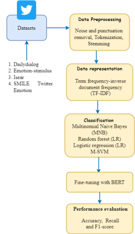
In this section, we outlined the proposed solution for tweet classification and sentiment interpretation. It is essentially a two-stage pipeline, as illustrated in Figure 1. The first stage comprises a series of pre-processing processes that convert Twitter jargon into plain text, such as emoji’s and emoticons. The second stage is a classification scheme based on an M-BERT language model pre-trained on a single text corpus. This step entails the processing of the processed data. To classify five emotional states, we employ the TF-IDF (term frequency inverted text frequency) method. Vectorised terms are used to prepare a data set and regular expressions. Experts classify sentences into five types of sentiments: surprise, sadness, anger, fear, and happiness.
Figure 1. Process flow of two-stage pipeline of the system
3.1 Dataset description
After determining the emotional model, acquiring data specific to the course is the next important phase in identifying emotions from the text. There are several freely accessible, structured, annotated ED databases for testing. The data collection we will use is publicly accessible in this article. The Emotion-Text Dataset was 70% divided into training, and 30% tested. The dataset was combined from regular dialogue [23], isear [24], and emotional stimulus [25] to include a balanced dataset containing five different labels: joy, sadness, anger, fear, and surprise, and even the Smile dataset [26] includes other annotations of disgust, anger, sadness, happiness, and surprise. We composed mostly the texts of short messages and speeches.
3.2 Data pre-processing
Before applying the final sentiment analysis techniques, we execute the pre-processing phase. We used the following phases in the typical production process: The raw Twitter data usually includes unique emojis (e.g. #,?...).
1. Stop word Removal: stop words are sometimes used in the real meaning of a document that has little contribution (e.g. a, and, the, etc.). Then the removal of the stop word is performed.
2. Stemming: In addition, variations of a base term, such as stems, are used in most sentences. Therefore, the variants of words are often simplified to their root shape as stems (for example, "joyful" or "joyful" are reduced to "joy" stems). This is used for the function of Porter’s stemming algorithm.
3. Tokenization: The word is further separated into actual token words. These are both measures for cleaning the data and preparing it for further study.
3.3 Feature extraction or data (text) representation
TF-IDF: Statistical algorithms use mathematics to understand model machine learning. Although numbers function in mathematics, we first have to translate the document into numbers to allow mathematical algorithms to perform for text. To achieve this, there are three major approaches: Word Bag, TF-IDF, and Word2Vec. We used the TF-IDF system in this current study.
3.4 Classifier model
Because the analysis has a multi-class dilemma, we discovered that the multi-class text classification of the NB is superior to multinomial Naive Bayes (MNB).
Naive Bayes: The Naive Bayes (NB) classification has proven efficient for the study of sentiments. The principle behind the Bayes classification is the Bayes theorem to evaluate the probability of a feature vector of a class S.
$P(s \mid \vec{f})=\frac{P(\vec{f} \mid s) P(s)}{P(\vec{f})}$ (1)
The simplistic (name-listed) hypothesis is that all characteristics are independent of each other. Because of this supposition, and since P(f~) for all groups is the same, equation 2 can find the most likely class ~ s for a variable f~.
$\hat{s}=\arg \max P(s) \prod_{j=1}^{n} P\left(f_{j} \mid s\right)$
$s \in S$ (2)
Random Forest: It is a controlled classifier using a combination of learning technology in various training stages of decision-making bodies. The number of trees calculated the exactness of the classifier and increased the number of trees in the method to improve the system's precision. The Decision Tree is a structure with a monitoring testing dataset, and these trees generate rules for each class during training. They then used these principles as the evaluation data parameters that may vary from the training data collection. The random forest selects some features from all the features provided for each class at the beginning of the algorithm. The test dataset progresses through every tree specified during the learning stage. We then assessed the target votes by comparing each prediction target. The Random Forest algorithm has a benefit that was never generated compared to the results of the classification. Since the problem model is often a minor error in the Random Forest, we may also use this technology for regression, classification, and extraction tasks.
Logistic regression: It is a regression class used to forecast the dependent variable of an independent variable. The Dual logistic regression is where the dependent variable has two types. If the dependent variable has over two types, the logistic regression is multinomial. If the vector type is classified, then the ordinal logistic regression (OLS). Turn the dependent variable into the logic function to achieve the highest probability estimate. Logit is primarily a natural log of the variable which shows whether the occurrence will take place. Ordinal logistic regression does not assume a linear association between the contingent and the independent variable.
Multi-Support Vector Machine (MSVM): We monitor it using a machine learning algorithm used in classification and regression models. Compared with artificial neural networks, the SVM method provides better classification outcomes since it has a plethora of generalizations that prevent the algorithm from overfitting. The SVM is a versatile machine that learns to handle nonlinear data for regression and classification problems with an appropriate kernel feature. The two key hyper-parameters are C and γ in the SVM algorithms. We should adjust the hyper-parameters before training the model. We used the overall parameters to train the SVM according to the training information. The model on the validation collection is then checked. Finally, on the reference dataset, we tested the model. We used linear, polynomial and RBF as an SVM kernel and as a decision function one-on-one (ovo). After a comparative analysis, when attempting various parameters, such as C, γ and kernel. In training, validation and testing, we have observed that classifiers of almost all kinds of combinations end up the same. It’s because SVM was first designed for binary classification, which is an issue for multi-class classification. We use ovo, which means they are binary versus one. We have, however, noticed that SVM could not be so appropriate for this task. The outcome shows that data precision is not so satisfactory. Following specific exploration, we found three multi-class problem-solving systems. They are ovr (one vs residue), M (M-1)/2 and expand the SVM formula.
The adapted classifier has the following form.
$f_{t a r}(x)=\sum_{k=1}^{M} \tau^{k} f_{\operatorname{src}}^{k}(x)+\Delta f(x)$ (3)
where, $\tau^{k} \in(0,1)$ is the weight of each base classifier $f_{\operatorname{src}}^{k}(x)$, $\Delta f(x)$ is the perturbation function that is learnt from a small set of labelled target-domain data in $D_{\text {tar }}^{l}$. As shown in the study [27] it has the form:
$\Delta f(x)=w^{T} \phi(x)=\sum_{i=1}^{N} \alpha_{i} y_{i} K\left(x_{i}, x\right)$ (4)
where, $w=\sum_{i=1}^{N} y_{i} y_{i} \phi\left(x_{i}\right)$ is the model parameters under which the labelled example $D_{\text {tar }}^{l}$ and $a_{i}$ is to be measured and where is the target-domain case ith-labeled function coefficient. Non-linear mapping of features often caused the kernel function as $K(., .) \equiv \phi(.)^{T} \phi(.)$. They learnt it $\Delta f(x)$ in regularized scientific risk minimization [28]. The adapted classifier $f_{\text {tar }}^{(x)}$ studied in this context seeks to minimize the classification error in the target-domain examples mentioned and the distance from the basic classifiers $f_{S r c}^{k}(x)$ to achieve a more bias-variance. We use an expanded multi-classifier adjust mechanism suggested by Yang & Hauptmann [29] to enable the weight controls $\left\{\tau^{k}\right\}_{k=1}^{M}$ based on the weight output of the limited range of target-domain examples in the base classifiers $f_{S r c}^{k}(x)$ to be automatically learned. To do this, the adaptive classifier is now written as:
$\min _{w, \tau, \xi} \frac{1}{2} w_{w}+\frac{1}{2} B(\tau)^{T} \tau+C \sum_{i=1}^{N} \xi_{i}$
s.t. $y_{i} \sum_{k=1}^{M} \tau^{k} f_{s r c}^{k}(x)+y_{i} w^{T} \phi\left(x_{i}\right) \geq 1-\xi_{i}$
$\xi_{i}^{m} \geq 0, \forall\left(x_{i}, y_{i}\right) \in D_{s r c}$ (5)
where, $\frac{1}{2}(\tau)^{T} \tau$ the total input of the base classifiers is steps, is added to the regularized loss minimization process. This objective function aims to prevent dependency and over-complexity $\Delta f(.)$ on the basic category. Parameter B balances the two targets. By rewriting the objective function as a Lagrange (primal) function minimization problem and setting its derivative w, and ξ to zero, we have:
$w=\sum_{i=1}^{N} \alpha_{i} y_{i} \phi\left(x_{i}\right) \tau^{k}=\frac{1}{B} \sum_{i=1}^{N} \alpha_{i} y_{i} f_{s r c}^{k}\left(x_{i}\right)$ (6)
where, $\tau^{k}$ a weighted sum $y_{i} f_{s r c}^{k}(x i)$ and the classification performance of the target domain. Consequently, if we classify the labelled destination domain info well, we have allocated more massive base classifiers. With the new decision function provided (3), (4) and (6) now:
$f_{t a r}(x)=\frac{1}{B} \sum_{k=1}^{M} \sum_{i=1}^{N} \alpha_{i} y_{i} f_{\operatorname{src}}^{k}\left(x_{i}\right) f_{\operatorname{src}}^{k}(x)+\Delta f(x)$
$=\sum_{i=1}^{N} \alpha_{i} y_{i}\left(K\left(x_{i}, x\right)+\frac{1}{B} \sum_{k=1}^{M} f_{\operatorname{src}}^{k}\left(x_{i}\right) f_{\operatorname{src}}^{k}(x)\right)$ (7)
Compared with (7) a regular SVM model $f(x)=\sum_{i=1} a_{i} y_{i} K\left(x_{i}, x\right)$, this multi-classification adaptation model may be interpreted as applying additional features to the projected labels of the basic classifiers in the target domain. The scalar B combines the influence of the initial characteristics and more features according to this interpretation.
3.5 Fine-tuning BERT for sentiment analysis
BERT is a pre-training technique created by Google for NLP (Natural Language Processing) [30]. We designate BERT to pre-train deep bidirectional representations from an unlabeled document by shaping both left and right instances in both layers. As a result, only one additional output layer will complete the pre-trained BERT model to construct state-of-the-art models for various tasks, including answering questions and language inference, without significant task-related changes to the design, as seen in Figure 2.
We used the library of transformers and designed a model of BERT. But it wasn’t appropriately prepared because of some unknown issue. We moved and developed the model into another library named Ktrain. "Ktrain is a lightweight wrapper for the TensorFlow Keras (and other libraries) deep learning library to support the development, training, and deployment of neuronal network and other learning systems models. We used BERT from the Ktrain library.
Figure 2. Architecture of BERT model
Proposed fine tuning of modified BERT: When we evaluated the efficiency of the MBERT to that of a baseline model that uses a TF-IDF vectorizer and an MSVM classifier. The transformers library allows us to fine-tune the cutting-edge BERT model fast and inexpensively, yielding an accuracy rate higher than the baseline method.
Step 1: Simply install the Hugging Face Library
This includes PyTorch variants of BERT (from Google), GPT, and pre-trained network weights.
Step 2: Tokenization and Input Formatting
Prior to actually tokenizing our content, we will perform some basic text processing, such as extracting entity mentions (e.g., @united) and even some special characters. Since BERT was trained with whole sentences, the level of processing here is substantially lower than in previous approaches. We must utilize the tokenizer given by the library in order to apply the pre-trained BERT.
This is due to the fact that
Furthermore, we must add special tokens to the beginning and end of each sentence, pad and truncate all sentences to a single consistent length, and specifically define which tokens are padding tokens using the "attention mask."
Step 3: Train Our Model
BERT-base is made up of 12 transformer layers, each of which takes in a list of token embeddings and outputs the same number of word embedding with the same hidden size (or dimensions). The output of the [CLS] token's final transformer layer is being used as the sequence's features to feed a classifier.
The Bert for Sequence Classification class in the transformers library is intended for classification tasks. Therefore, we will develop a new class in order to specify our own classifiers. In the following section, we will build a Bert Classifier class that uses a BERT model to extract the last hidden layer of the [CLS] token and a single-hidden-layer feed-forward neural network as the classifier.
Step 4: Optimizer and Learning Rate Scheduler
We'll need an optimizer to fine-tune our Bert Classifier. We set batch size to be 32, learning rate to 5e-5, and number epochs be 4.
Step 5: Build a Training Loop
For 4 epochs, we will train the Bert Classifier. We will train the model and evaluate its performance on the validation set at the end of each epoch. Compute the average loss across all training data. After each training epoch, evaluate the performance of the model on our validation set and computes the accuracy rate.
We present the test results in this segment and equate our proposed SVM adaptation scheme with a collection of 3 data sets together with a BERT model of twitter. In addition, we examine the impact on classification efficiency of different sizes of the labelled target domain results. Python versions 3.6 and 3.7 were used for testing, as well as MATLAB R2019b or later, Statistics and Machine Toolbox, and Text Analytics Toolbox for algorithm implementation.
DailyDialog dataset: There are 13,118 multi-turn dialogues in the DailyDialog dataset. They also counted the average speaker turns and tokens to provide the dataset with an overview. The statistics resulting are seen in the following table. The numbers we can see are about eight turns for the speaker and around 15 turns for each utterance, as seen in Table 1.
Table 1. Basic statistics of DailyDialog
|
Content |
Size |
|
Total Dialogues |
13,118 |
|
Average Speaker Turns Per Dialogue |
7.9 |
|
Average Tokens Per Dialogue |
114.7 |
|
Average Tokens Per Utterance |
14.6 |
Emotion-stimulus dataset: The Emotion-Stimulus Dataset is both emotional and stimulating, with the help of the emotionally oriented FrameNet frame. Their emotional tag included 820 penalties for both reason and emotion and 1594 sentences. Categories: happiness, sadness, anger, fear, surprise, disgust, and shame. It includes 2,414 XML file formats.
ISEAR (International Survey on Emotion Antecedents and Reactions) dataset: A commonly used ISEAR data collection evaluates the suggested system. It has seven fundamental emotions, such as anger, disgust, fear, guilt, joy, shame, and sadness. Each term has a group mark, while the number of phrases is 7666, with 1096 individuals filling the survey questionnaires. Table 2 shows one example phrase from the category of anger before and during stemming. The words implying the emotion of anger are unclear. In addition, the volumes are minimal.
Table 2. Sample sentence from the anger category before and after stemming
|
When I was driving home after several days of hard work, there á was a motorist ahead of me who was driving at 50 km/hour and á refused, despite his low speed to let me overtake. |
|
When wa drive home after sever dai of hard work there wa motorist ahead of me who wa drive at km hour and refusdespit hi low speeed to let me overtak. |
SMILE Twitter Emotion dataset: A surprising class imbalance is seen by the distribution of emotional annotations, with 30.2% of tweets being happy and the rest of the emotions seldom shown in museum results. There are still several emotionally unrelated tweets (41.8%). An intuitive theory is that Twitter users prefer to share optimistic and appreciative memories with their museums and fear derogatory feedback. The museum data emotion allocation to our general-domain data may also be illustrated by contrasting the optimistic sampling ratio of individual emotions to our general-domain source data. In this analysis, we coupled the dataset with everyday dialogue, sadness, rage, fear, and neutrality to construct a healthy dataset with five labels. The texts comprise mostly short messages and speeches in dialogues. Table 3 lists all the four datasets' information along with their size and emotion categories.
Table 3. Summary of four datasets
|
Dataset |
Content |
Size |
Emotion categories |
|
Dailydialog |
Dialogues |
102k sentences |
Neutral, joy, surprise, sadness, anger, disgust, fear |
|
Emotion-stimulus |
Dialogues |
2.5k sentences |
Sadness, joy, anger, fear, surprise, disgust |
|
Isear |
Emotional situations |
7.5k sentences |
Joy, fear, anger, sadness, disgust, shame, guilt |
|
SMILE Twitter Emotion |
Emotion annotations |
3,085 tweets |
Anger, disgust, happiness, surprise, sadness. |
Performance evaluation: We used both classifiers for the grouping. Real-time data labels have been allocated based on the likelihood of emotional term frequency, predefined in [6], which can then evaluate the classifiers. Their e valuation in terms of performance metrics is conveyed. Accuracy, Recall, and the F1-scoreare the metrics used for classification efficiency evaluations. Table 4 provides F1-score and Accuracy of combined dataset for five types of ML approaches.
Accuracy $($ Acc $)=\frac{\text { Correctly predicted observations }}{\text { Total number of observations }}$ (8)
Recall $=\frac{\text { Correctly predicted positive observations }}{\text { Total positive observations }}$ (9)
$\mathrm{F} 1-\mathrm{score}=\frac{2}{\frac{1}{\text { Precision }}+\frac{1}{\text { Recall }}}$ (10)
Table 4. F1-Score, Accuracy of combined dataset
|
Type of ML approach |
F1-score |
Accuracy |
|
Multinomial Naive Bayes (MNB) |
67.02 |
67.88 |
|
Random Forrest (RF) |
63.72 |
64.12 |
|
Logistic Regression (LR) |
69.35 |
70.12 |
|
Multi-SVM |
72.71 |
73.24 |
|
Modified BERT (Our work) |
97.63 |
98.91 |
Figure 3. Comparison for performance for 4 machine learning model
From Figure 3 it is clear that Our Modified BERT is showing better performance as compared to all other four ML approaches. Our Modified BERT has a highest F1-score of 97.63%, compared with the least F1-score of 63.72% in case of Random Forest, and similarly Our Modified BERT shows highest accuracy of 98.91% as followed by the MNB of 67.88%, RF of 64.12% and LR of 70.12% models and multi-SVM of 73.24%. This shows that for both the two-performance metrics (i.e., F1-score and accuracy), Our Modified BERT outperforms as related to four ML approaches.
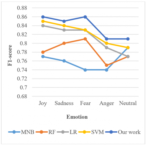
The effect of fine tuning with modified (M-BERT)-Our work on machine learning models: As illustrated in Figure 4, our model outperforms the original BERT model with the help of modified (M-BERT). The modified (M-BERT) F1-score is higher than other models (i.e., MNB, LR and RF), particularly in the joy and fear emotions. There are fewer samples of fear and anger in our dataset than in the others, and the improvement is mainly in these two types of emotions. As a result, the performance includes evidence of our fine-tuning and combination approaches to dealing with the unbalanced dataset.
Figure 4. The effect of modified (M-BERT) on machine learning models on F1-score
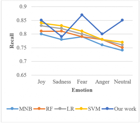
As illustrated in Figure 5, our model outperforms the original BERT model with the help of modified (M-BERT). The modified (M-BERT) recall is higher than other models (i.e., MNB, LR and RF), particularly joy and fear emotions. There are fewer samples of fear and anger in our dataset than in the others, and the improvement is mainly in these two types of emotions. As a result, the performance shows the relevance of our fine-tuning model correctly predicting the overall number of emotions.
Figure 5. The effect of modified (M-BERT) on machine learning models on recall
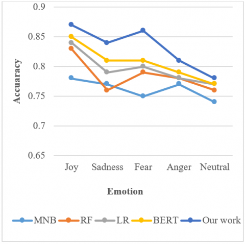
As illustrated in Figure 6, our model outperforms the original BERT model with the help of modified (M-BERT). The modified (M-BERT) model outperforms the other four models, particularly Joy, Sadness, and Fear emotions. There are many fewer neutral examples in our collection than in the others, and the improvement is primarily in this type of emotion. As a result, the performance shows the relevance of our fine-tuning model correctly classifying the overall number of emotions.
Figure 6. The effect of modified (M-BERT) on machine learning models on accuracy
The primary objective of this work was to introduce an appropriate solution for Twitter sentiment analysis based on the BERT language model. It was designed as a two-step pipeline, with the first step involving a series of pre-processing procedures to convert Twitter jargon, including emoji’s and emoticons, into plain text, and the second step utilizing a version of BERT that was pre-trained on plain text to fine-tune and classify the tweets based on their polarity. The classification of emotions has a wide range of applications. It is of great importance to give a precise and effective classification scheme. We utilize datasets in conjunction with the Dailydialogue, ISEAR emotion stimulus, and SMILE Twitter Emotion with many classifications using machine-learning algorithms such as MNB, Random Forest, LR, and M-SVM. A four n-fold cross-validation technique compares their classification performance. Although we are using a publicly available BERT pre-trained model, the outcome is significant. Our fine-tuning MBERT with Multi-SVM methods improved our model's performance in the unbalanced dataset and showed our model's performance on the multi-label and multilingual sentiment analysis challenge. We can reach relatively close performance by layering a simple one-hidden-layer neural network classifier on top of BERT and fine-tuning MBERT, which is 24.92% better than the baseline BERT technique. An amazing result with a minimal amount of data was achieved in a short amount of time.
[1] Edison, M., Aloysius, A. (2017). Lexicon based acronyms and emoticons classification of sentiment analysis (SA) on big data. International Journal of Database Theory and Application, 10(7): 41-54. https://doi.org/10.14257/ijdta.2017.10.7.04
[2] Airton, J., Nadia, F., Thierson, C., Celso, J. (2021). Sentiment analysis with genetic programming. Information Sciences, 562: 116-135. https://doi.org/10.1016/j.ins.2021.01.025
[3] Alexander, B. (2018). Positive vs. Negative feedback mechanisms. Science Trends. https://doi.org/10.31988/SciTrends.41706
[4] Morgan, B., D’Mello, S. (2013). The effect of positive vs. negative emotion on multitasking. In Proceedings of the Human Factors and Ergonomics Society Annual Meeting. 57: 848-852. https://doi.org/10.1177/1541931213571184
[5] Wang, R., Ridley, R., Qu, W., Dai, X. (2021). A novel reasoning mechanism for multi-label text classification. Information Processing & Management, 58(2): 102441. https://doi.org/10.1016/j.ipm.2020.102441
[6] Batista dos Santos, V., Merschmann, L.H.D.C. (2020). Metalearning applied to multi-label text classification. In XVI Brazilian Symposium on Information Systems, pp. 1-8. https://doi.org/10.1145/3411564.3411646
[7] Li, X., Li, J., Wu, Y. (2015). A global optimization approach to multi-polarity sentiment analysis. PloS One, 10(4): e0124672. https://doi.org/10.1371/journal.pone.0124672
[8] Wang, W., Li, B., Feng, D., Zhang, A., Wan, S. (2020). The OL-DAWE model: Tweet polarity sentiment analysis with data augmentation. IEEE Access, 8: 40118-40128. https://doi.org/10.1109/ACCESS.2020.2976196
[9] Naicker, N., Adeliyi, T., Wing, J. (2020). Linear support vector machines for prediction of student performance in school-based education. Mathematical Problems in Engineering, pp. 1-7. https://doi.org/10.1155/2020/4761468
[10] Pranckevičius, T., Marcinkevičius, V. (2017). Comparison of naive bayes, random forest, decision tree, support vector machines, and logistic regression classifiers for text reviews classification. Baltic Journal of Modern Computing, 5(2): 221. https://doi.org/10.22364/bjmc.2017.5.2.05
[11] Li, M., Ch’ng, E., Chong, A.Y.L., See, S. (2018). Multi-class Twitter sentiment classification with emojis. Industrial Management & Data Systems, 118(9): 1804-1820. https://doi.org/10.1108/IMDS-12-2017-0582
[12] Xu, L., Qiu, J. (2019). Unsupervised multi-class sentiment classification approach. KO KNOWLEDGE ORGANIZATION, 46(1): 15-32. https://doi.org/10.5771/0943-7444-2019-1-15
[13] Singla, S., Kumar, V. (2020). Multi-Class sentiment classification using machine learning and deep learning techniques. International Journal of Computer Sciences and Engineering, 8(11): 14-20. https://doi.org/10.26438/ijcse/v8i11.1420
[14] Liu, Y., Bi, J.W., Fan, Z.P. (2017). Multi-class sentiment classification: The experimental comparisons of feature selection and machine learning algorithms. Expert Systems with Applications, 80: 323-339. https://doi.org/10.1016/j.eswa.2017.03.042
[15] Zainuddin, N., Selamat, A., Ibrahim, R. (2018). Hybrid sentiment classification on twitter aspect-based sentiment analysis. Applied Intelligence, 48(5): 1218-1232. https://doi.org/10.1007/s10489-017-1098-6
[16] Wang, R., Li, Z., Cao, J., Chen, T., Wang, L. (2019). Convolutional recurrent neural networks for text classification. In 2019 International Joint Conference on Neural Networks (IJCNN), pp. 1-6. https://doi.org/10.1109/IJCNN.2019.8852406
[17] Vieira, J.P.A., Moura, R.S. (2017). An analysis of convolutional neural networks for sentence classification. In 2017 XLIII Latin American Computer Conference (CLEI), pp. 1-5. https://doi.org/10.1109/CLEI.2017.8226381
[18] Bhatta, J., Shrestha, D., Nepal, S., Pandey, S., Koirala, S. (2020). Efficient estimation of Nepali word representations in vector space. Journal of Innovations in Engineering Education, 3(1): 71-77. https://doi.org/10.3126/jiee.v3i1.34327
[19] Subakan, C., Ravanelli, M., Cornell, S., Bronzi, M., Zhong, J. (2021). Attention is all you need in speech separation. In ICASSP 2021-2021 IEEE International Conference on Acoustics, Speech and Signal Processing (ICASSP), pp. 21-25. https://doi.org/10.1109/ICASSP39728.2021.9413901
[20] Devlin, J., Chang, M.W., Lee, K., Toutanova, K. (2018). Bert: Pre-training of deep bidirectional transformers for language understanding. arXiv preprint arXiv:1810.04805.
[21] Wang, T., Yang, X., Ouyang, C., Guo, A., Liu, Y., Li, Z. (2018). A multi-emotion classification method based on BLSTM-MC in code-switching text. In CCF International Conference on Natural Language Processing and Chinese Computing, pp. 190-199. https://doi.org/10.1007/978-3-319-99501-4_16
[22] Lee, S.Y.M., Wang, Z. (2015). Multi-view learning for emotion detection in code-switching texts. In 2015 International Conference on Asian Language Processing (IALP), pp. 90-93. https://doi.org/10.1109/IALP.2015.7451539
[23] Li, Y., Su, H., Shen, X., Li, W., Cao, Z., Niu, S. (2017). Dailydialog: A manually labelled multi-turn dialogue dataset. arXiv preprint arXiv:1710.03957.
[24] Scherer, K.R., Wallbott, H.G. (1994). Evidence for universality and cultural variation of differential emotion response patterning. Journal of Personality and Social Psychology, 66(2): 310-328. https://doi.org/10.1037/0022-3514.66.2.310
[25] Ghazi, D., Inkpen, D., Szpakowicz, S. (2015). Detecting emotion stimuli in emotion-bearing sentences. In International Conference on Intelligent Text Processing and Computational Linguistics, pp. 152-165. https://doi.org/10.1007/978-3-319-18117-2_12
[26] Ramalingam, V.V., Pandian, A., Jaiswal, A., Bhatia, N. (2018). Emotion detection from text. In Journal of Physics: Conference Series, 100(1): 012027. https://doi.org/10.1088/1742-6596/1000/1/012027
[27] Xu, S.X., Yang, J., Tang, S., Zhang, Y.D. (2011). A pseudo relevance feedback based cross domain video concept detection. In Proceedings of the Third International Conference on Internet Multimedia Computing and Service, pp. 21-25. https://doi.org/10.1145/2043674.2043681
[28] Yang, J., Tong, W., Hauptmann, A.G. (2012). A framework for classifier adaptation for large-scale multimedia data. Proceedings of the IEEE, 100(9): 2639-2657. https://doi.org/10.1109/JPROC.2012.2204009
[29] Yang, J., Hauptmann, A.G. (2008). A framework for classifier adaptation and its applications in concept detection. In Proceedings of the 1st ACM International Conference on Multimedia Information Retrieval, pp. 467-474. https://doi.org/10.1145/1460096.1460171
[30] Bao, H., Dong, L., Wei, F. (2021). BEiT: BERT Pre-Training of Image Transformers. arXiv preprint arXiv:2106.08254.