Krishna Chythanya Nagaraju* | Cherku Ramesh Kumar Reddy
© 2021 IIETA. This article is published by IIETA and is licensed under the CC BY 4.0 license (http://creativecommons.org/licenses/by/4.0/).
OPEN ACCESS
A reusable code component is the one which can be easily used with a little or no adaptation to fit in to the application being developed. The major concern in such process is the maintenance of these reusable components in one place called ‘Repository’, so that those code components can be effectively identified as well as reused. Word embedding allows us to numerically represent our textual information. They have become so pervasive that almost all Natural Language Processing projects make use of them. In this work, we considered to use Word2Vec concept to find vector representation of features of a reusable component. The features of a reusable component in the form of sequence of words are input to Word2Vec network. Our method using Word2Vec with Continuous Bag of Words out performs existing method in the market. The proposed methodology has shown an accuracy of 94.8% in identifying the existing reusable component.
repository, Word2Vec, search, code component, neural network
The inevitable scenario in the fast code development situations is writing the same code over and over again. In order to reduce time, effort, also to drastically improve the efficiency of development process, almost all organizations now prefer to have a mono repository to maintain the reusable code components. A reusable code component is the one which can be easily used with a little or no adaptation to fit in to the application being developed. Component Based Software Engineering (CBSE) is on high demand giving major benefits of less workforce needed besides lines of code to be developed for an application would be considerably reduced using on the shelf components. The major concern in such process is the maintenance of these reusable components in one place called Repository, so that those code components can be effectively identified as well as reused. Hence, the way Repository is maintained affects the software development process and the success of organization that is practicing CBSE. In case of searching for a required component if the repository is of small size, it would be a simple task but in case where repository consists of thousands of components, searching a required component is also a complex problem that attracted many researchers to work on.
Word embedding allows us to numerically represent our textual information. They have become so pervasive that almost all Natural Language Processing projects make use of them. Even though each line of a code component is not exactly as a natural language sentence, yet the basic building blocks are from natural language and does has some contextual meaning among the words we use in every line of code snippet that is developed. Hence in this work we considered to use Word2Vec concept to develop word embeddings. Word embedding algorithms like Word2Vec are unsupervised feature extractors of words.
To properly understand the context of the word used one need to make use of word embeddings. The vocabulary of document considered is represented in the vector form using word embeddings that enable capturing of context. This context can be used for identifying the required document more accurately as compared to general process of document or file identification from large corpus of dataset.
Mikolov et al. [1] proposed one of the best mechanisms of word embedding called Word2Vec with an objective to maintain words with similar context to be occupying in close spatial proximity. Generally, Word2Vec models are shallow two-layered neural network architectures. Comparison becomes easy when something has magnitude & direction hence vector representation is considered for words as Vectors are something which has both magnitude & direction.
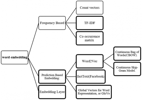
The simplest word embedding one can find is one hot vector encoding. Consider a set of words to be converted in to numerical representation so that same can be used as an input to a machine learning algorithm based model. Such model can be further used in recommendation systems. The simplest thing that can be done is giving numerical indexing to each word in word set we considered say like, 1,2,3…some 10,000. This can be further represented in binary format with all 0s except one bit as ‘1’ corresponding to the position of word in the vocabulary corpus we consider. For example [0,0,0,..1,0,0,0..0,0] etc. But this representation has a fundamental problem of not considering the contextual information among a sequence of words which actually plays in understanding the actual semantics of those set of words or in simple processing of natural language. Another biggest problem would be, one hot encoding is resulting in mostly sparse vector representation. This results in poor memory utilization though they are quick and easy way to represent each word as real valued vectors. One hot encoding fares poorly in case of analogy based identification of word representation in natural language context. Also, the size of the vector here is directly proportional to the size of the vocabulary corpus considered. As size grows too large, indexing, searching would become a linear problem with more time consumption besides sparse space issue. As these word representations in numerical forms will be used as input for Neural Networks in process of predictions and comparisons, this would make Neural Networks to struggle in giving high performance or even in training. One of the simplest mechanisms if we want embedding of whole sentence instead of word would be averaging real values of words in sentence. The other advanced methods include Recurrent Neural Network (RNN) encoder-decoder models. The RNN models will build embedding of sentences reading word by word. The greater advantage of word embedding lies in generalization. The different types of word embeddings can be shown as in Figure 1 below. The representation in higher dimension vector space raises a question of dimensionality as, what is the accurate number of embedding dimensions that can solve the problem of context representation? This empirical question always needs look for a tradeoff between accuracy and computational complexity.
Figure 1. Different types of word embeddings
There are two main differences between Bag of Words (BoW) or Term Frequency-Inverse Document Frequency (TF-IDF) in keeping with word embedding:
BoW or TF-IDF creates one number per word while word embedding typically creates one vector per word.
BoW or TF-IDF is good for classification documents as a whole, but word embedding is good for identifying contextual content.
New avenues are being open for machine learning to process source code with ever growing demand of open source repositories. Attention based neural machine transition using encoder- decoder architecture is used to select relevant paths while decoding by representing code as an Abstract Syntax Tree (AST) in the work done by Alon et al. [2] named as code2seq model. The developing of natural language sequences from the code snippets is very useful in retrieval, summarization or documentation of code snippets. They have worked on two aspects – code summarization and code captioning but did not test it on code retrieval. Shido et al. [3] in their work entitled “Automatic source code summarization with extended tree-LSTM” have successfully implemented multi-way tree Long Short Term Memory to handle a node that has arbitrary number of children and their order in ASTs simultaneously.
In the work of Hussian et al. [4], they developed a CODESEARCHNET corpus besides throwing open CODE SEARCH-NET CHALLANGE. The corpus they developed was based on different open source code works and contains around six million functions belonging to different programming languages like Ruby, Java, GO, JavaScript etc. The researchers make use of ‘joint vector representation’ for code search. A neural system is implemented using joint embeddings of code and queries. Contextualization of token embedding was achieved using Neural Bag of Words architecture. Any how the underlying searching mechanism is of Elastic search which performs traditional keyword based search but representing rare terms was a thing missing in their work. They do raise a question of, “can we have similar to BERT pre training methods of Natural Language Processing for the encoders considered in work?”
In the work done by Akbar and Kak [5], they concentrated on mechanisms to impose ordering constraints using logic of Markov Random Fields (MRF) on the embedded word representations. During source code retrieval, while matching order of words in an enquiry with words sequence in a file, exploitation of semantic word vector generated using word2vec is done. In the literature, we can find several BoW based source code retrieval methods [6-13]. Authors have also reported using word2vec for software search [14-17], The researchers considered Correct at r C@r with abbreviation occurring in top r ranked positions and Pearson Correlation score to evaluate their work using popular data sets of Eclipse and AspectJ.
Emphasizing on the issue of handling mismatch in code search/retrieval using deep learning with Word2Vec was done by Van Nguyen et al. [16], in which the researchers combined Word2Vec with Revised Vector Space model for better code retrieval (rVSM). rVSM computes the weight for a word based on a new term frequency-inverse document frequency (tf-idf) formula and a new scoring scheme among the vectors that takes documents’ lengths into account. In their work they claim an API code example retrieval accuracy for rVSM + Word2Vec to be as 60.9 for top 5 recommended code snippets. We could get a better performance through our method than this for our data set as discussed in Results section at the end of this paper.
Sugatadasa et al. [18] have considered Legal Domain with 25000 legal cases collected from other research works, for document information retrieval. They proposed document embeddings system for legal domain based on TF-IDF with page ranking graph network and the same was used to train a neural network model in an incremental model. In the process they did not consider a specific legal case that is mentioned in another legal case a greater number of times, as it may be more significant for that case. By assigning weights to this most relevant case for the legal case under consideration more accurate interlinking is possible among the documents that may enhance the overall performance Li et al. [19] work on a structure driven method for information retrieval-based change impact analysis (SDM-CIA). This SDM CIA integrates both bag of words and word embedding models [20].
Though the main purpose of word2vec can be seen in word prediction yet in our case it acts as a proxy to learn vector notations of words which will be further used to represent the features of a reusable component and a repository is build based on collection of these vector notations. The weights obtained after training, between Input Layer and Hidden Layer are the values we plan to use to represent feature set of a reusable component. The flow chart of our idea is depicted in Figure 2 below.
Figure 2. The flow chart of methodology we followed
The algorithm followed in implementing this work is as shown below.
Algorithm 1_CR: Algorithm for component retrieval using Word2Vec-CBoW method (parameter1, parameter2.. .. parameter18):
Input: feature set consisting of 18 words, read from the user i.e. Parameter 1 to Parameter 18 as shown in parenthesis above.
Output: 1. If the component exists in Repository; it gives “component matches” message along with location of component to retrieve.
2. If the component doesn’t exist in the Repository, it gives a “Not Found” or error message and gives an option for user to upload the component.
Begin:
Step1: Read Fciß {f1,f2,f3,f4…f18};//18 features selected from GUI.
Step 2: Mß Fci//Trained Word2Vec-CBoW Neural network model given with input
Step 3: wviß M(fi) where i=1,2,3,4…18;// vector for each word in feature set is generated
miß mean(wvi), where i=1,2,3,4…18;// mean for each vector of word is calculated
MCß (Ʃi=1to 18mi) /18;// overall mean of all vectors generated for all features of a component
Step 4: Result = Search_AVL (Mc)// Searching for required component in AVL tree using Mc
4a: If the mean value matches with any node value in AVL tree,
Resultß Component Matches, its Location.
4b: If the mean value doesn’t match with any node of AVL tree constructed during building of Repository,
Result ß Not Found
Option to upload is given.
End.
In the above algorithm, Fci stands for the 18 features set of a component being searched. This is given as input by the user during searching for a reusable component. M is the trained Word2Vec-CBoW Neural Network model for which this Fci is given as input. The model finds word vectors of each word in the feature set like wv1,wv2…. wvi. wv18. The mean of each such generated word embedding vector is calculated in mi and Average of all 18 means of all 18 features is calculated in Mc. This value in Mc is given as input for search in AVLtree developed during building of repository to check whether the component already exists or not. Let us try to understand the logic behind word embedding and how this algorithm works with an example as discussed here after in this section.
In embeddings, dense vectors are used to represent words where in these vectors are in fact projection of word in continuous vector space. For applying neural networks on text data, data pre-processing is to be done to generate equivalent integer of unique value. This unique integer is further mapped in to a specific dimension real valued vector by embedding. The unique integer can be generated in preprocessing of data using Tokenizer API of Keras. The Embedding layer results in a 2D vector with each word being embedded uniquely from input sequence. Which means the word is represented as two real valued components in vector.
The mathematics behind word2vec is simple to understand. It takes one hot encoding of a specific word having “1” corresponding to that word index and all remaining index as zero. By multiplying weight matrix generated from random seed and updated over iterations of training by this input vector we would be extracting word index’s corresponding row. For example, considering a 4th word of a phrase [0 0 0 1] as shown below:
[0 0 0 1] * [24, 17, 6; 11, 8, 15; 16, 23, 43; 18, 9, 5]=[18,9,5]
In case of word2vec being implemented using Keras or Tensorflow this math work is done by a special layer called as “Ebedding Layer”. Consider the following 2 phrases simple training set for further understanding.
Happy to see you again; Hope to see you soon.
The above two phrases can be encoded by assigning a unique integer number based on order of appearance in training data set as [0, 1, 2, 3, 4]; [5, 1, 2, 3, 6]. The statement required for building embedding can be given as:
Embedding (7,2, input_length=5); where in 7 stands for number of unique words available in training set, the argument 2 indicates size of embedding vectors and the size of each input sequence is determined using argument input_length. The weights of embedding layer can be obtained after network is trained and for this example the size of matrix would be of 7X2. Let’s consider the embeddings as shown below in Table 1:
Table 1. Word Embeddings (Sample)
|
Index |
Embeddings |
|
0 |
[1.2,3.1] |
|
1 |
[0.4,4.1] |
|
2 |
[1.0,3.1] |
|
3 |
[0.3,2.1] |
|
4 |
[2.3,1.5] |
|
5 |
[0.9,1.7] |
|
6 |
[5.6,2.4] |
Accordingly, the second phrase in training can be represented as [[0.9,1.7], [0.4,4.1], [1.0,3.1], [0.3,2.1]].
For a given word say “soon”, the index is 6 and resulting one hot encoding of [0,0,0,0,0,0,1], multiplying this 1X7 matrix with embedding matrix of 7X2 we get required 2-Dimensional embedding, which can be seen in this case as [5.6,2.4]. The weight matrix of embedding gets initialized with random values and then optimized over training phases. The one hot encoding dimension of a given word would be consistent with the embedding matrix as it is dependent on size of word corpus of considered training set.
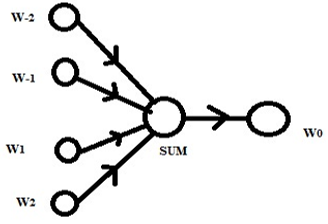
In general, the Continuous Bag of Words (CBoW) model predicts a current word based on the context of words given within a specific window size. The window size indicates how many context words should be considered. The CBOW model of Word2Vec can be depicted as shown in Figure 3 below.
Figure 3. Simple representation of CBOW model of Word2Vec. W-2, W-1, W1, W2 are context words for word W0
The underlying architecture of Word2Vec includes a Two-layer Neural Network for training that makes use of Back propagation algorithm. The Neural Network would have an Input Layer consisting of neurons in number equal to count of words in the vocabulary (V)followed by a Hidden Layer consisting of size equal to required dimensionality(N) of the resulting word vectors. The last layer would be an Output layer having neurons equal to input layer(V). The window size indicates the total words considered including center word for building context. In the above Figure 3, the window size considered is 5 for schematic purpose. The context window size considered for our work is 3 with vector dimensionality expected as 300. How we happened to fix with this 300 is explained in Results section below. The 300 means each word would be coded in to a vector size of 300 as shown in Figure 6 in following pages. The learning of parameters would be based on Backpropagation Algorithm and SoftMax activation function in output layer. The schematic representation of Neural Network model considered can be as shown in Figure 4 below. One hot encoding of word is considered as input with V dimensions that is equal to number of total words, which happens to be 18 in feature set. WVXN represents Weight matrix between input layer and Hidden layer whereas W’NXV represents weight matrix between hidden layer and output layer. As mentioned earlier that we use Word2Vec model as proxy as our concentration is on N dimension representation of word but not on the output layer.
Figure 4. The schematic view of Neural Network considered in Word2Vec model we used with window size=3
The work was carried out by considering a data set of 40000 components. The feature vector of reusable component constitutes of following information:
1.Operating System; 2. Programming Language; 3. Return Type; 4. No of Parameter 5. Type of Parameters; 6. Recursion; 7. Development Model; 8. Already Modified; 9. Time Complexity; 10. Space Complexity; 11. Reusability; 12. Well Documented; 13. Reliability; 14. Risk Factor; 15. Uploaded file type; 16. Data info; 17. Domain; 18. Lines of Code; 19. License; 20. Name of Program.
Each component is represented using a feature vector of 20 features set. For training purpose of Neural Network only 18 features were considered as “name of the program” (20th feature) and “licensing” (19th features) were not exactly contributing to identification of component very specifically. The feature vector is a collection of specific words which clearly distinguishes a code component. The considered 18 features are converted to vectors, which further will be given as input to neural network.
The following is a sample entry of one reusable component’s feature set as given by a user, let’s call it Fc:
1.Linux; 2. Ruby; 3. Derived data type; 4. Zero; 5. User defined data type; 6. Non recursive; 7.RAD; 8. Yes; 9. Nlogn; 10. One; 11. Fully reusable; 12. Excellent; 13. Up to Eighty; 14. High risk; 15. Code; 16. File input; 17. Banking; 18. Up to hundred.
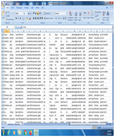
All the feature set of 40000 components considered is stored in a CSV file as shown in Figure 5 below, where each row indicates one component’s feature vector. Using Word2Vec technique the vector representation of each word is identified and these values are averaged to find equivalent vector value of one row, which is equal to the vector value representation of one component. The components are represented as a single mean value of word vector generated for features considered. These mean values are stored in an AVL tree data structure at the time of creation of repository.
Figure 5. Snapshot of dataset used in csv file format for training
When the user wants to search for a specific component, the user is asked to select the features of the component he is looking for, from the dropdown list created for each feature element in the GUI that is created using Tkinter. This leaves no scope for user to enter random data. Thus, makes it easy to handle data avoiding any necessity of cleaning and all fields are made mandatory so that no null values are taken. The entered feature set is a collection of words so using the already trained model the average value of vector representation of this collection of words is considered. The resulting average value now indicates the vector value of the component being search. Using AVL tree this value is simply checked whether exists in the repository or not. If it is there it means the required component exists else it means, the required component being searched for is not available in the component repository. For the purpose of experimentation, we have collected many code components from different resources on line such as sourceforge.net, Github etc. sites and as our methodology is completely new it requires building own repository.
Let us consider for step 1 the input is given as shown in example earlier called as Fc for the algorithm 1 described above. This is fed as an input to the pre trained model M generating word vector of each feature.
1.Linux 2.Ruby 3.Derived data type 4.zero 5.User defined data type 6.Non recursive 7.RAD 8.Yes 9.Nlogn 10.One 11.Fully reusable 12.Excellent 13.Up to Eighty 14.High risk 15.Code 16.File input 17.Banking 18.Up to hundred.
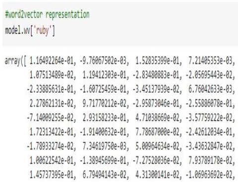
The vector representation of a word indicating “Language” feature of a specific component as considered in Fc, which is “Ruby” was observed to be as shown in Figure 6 below:
Figure 6. Sample 300-dimension vector generated for a Word of “ruby” indicating “Language” feature of a component
(Owing to space only a part of vector shown)
The values in the array in above figure indicate the 300 dimensions representation of word representing one feature of the component. This also signifies that we considered 300 neurons in the hidden layer of Word2Vec neural network. These hidden layer neurons are trained using back propagation algorithm. The authors of this work have done empirical study using size as 50,100,200,300,400 and the results obtained showed that when the size considered is 300 the model was giving better accuracy and hence, we stick on to 300-dimension vector representation.
Table 2 shows mean values obtained for the vector representation of each word in the feature set consisting of 18 features as shown in second column of table for the component being searched for. The mean value of all these 18 values is observed to be -0.007391004. This value now represents one reusable component.
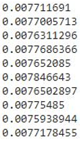
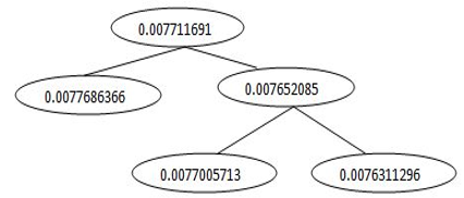
The mean value of vector generated for all words of the feature set would be a value of -0.007391004. This becomes the first node in the AVL tree at the time of repository creation and further values of second, third components etc. would be inserted under the root node and height balancing of AVL tree happens. While searching, this value generated like -0.007391004 is then checked for its availability in the repository built using AVL tree. The Figure 7 represents word vectors generated for features of first component considered from training set as shown in Figure 5. The mean value of each vector generated for each feature is calculated and further mean value of all such 18 features is calculated as explained in step 2 and step 3 of algorithm 1 above. This final mean value becomes the representation of a single component. Figure 8 shows the mean value of each component that would be stored in AVL tree. Owing to space constrains only values of a few (10) components are being shown in Figure 8. This means 0.007711691 value now represents first component as shown in first row of CVS file in Figure 5 and 0.0077005713 represents second component from Figure 5 and so on.
Considering inserting of first 5 values from the above mean values in to the AVL tree, the generated AVL tree after height balancing looks as in Figure 9.
Figure 7. Generated vector representation of features belonging to first component (Fc) from training set shown in Figure 5
Table 2. The table shows mean values of vectors generated by Word2Vec of each feature element for a component being searched for
|
Sl.No. |
Feature |
Sample Considered |
Mean of Vector generated |
|
Feature1 |
Operating System |
Linux |
-0.0068095303 |
|
Feature 2 |
Programming Language |
Ruby |
-0.006214711 |
|
Feature 3 |
Return Type |
Derived data type |
-0.0069797197 |
|
Feature 4 |
No.Of Parameters |
zero |
-0.0070498325 |
|
Feature 5 |
Type of Parameters |
User defined data type |
-0.007185216 |
|
Feature 6 |
Recursion |
Non recursive |
-0.0070020645 |
|
Feature 7 |
Development Model |
RAD |
-0.0056332634 |
|
Feature 8 |
Already Modified |
Yes |
-0.0066335257 |
|
Feature 9 |
Time Complexity |
n log n |
-0.0056920093 |
|
Feature 10 |
Space Complexity |
One |
-0.0058320006 |
|
Feature 11 |
Reusability |
Fully reusable |
-0.007200637 |
|
Feature 12 |
Well Documented |
Excellent |
-0.0071973926 |
|
Feature 13 |
Reliability |
Up to Eighty |
-0.00783842 |
|
Feature 14 |
Risk Factor |
High risk |
-0.008600807 |
|
Feature 15 |
Uploaded file type |
Code |
-0.008872024 |
|
Feature 16 |
Data info |
File input |
-0.009424939 |
|
Feature 17 |
Domain |
Banking |
-0.009272366 |
|
Feature 18 |
Lines of Code |
Upto hundred |
-0.009599611 |
Figure 8. Mean values calculated for word vectors of 10 components considered for training using CSV file as shown in Figure 5
Figure 9. AVL Tree generated after insertion of mean values of vector representation for 5 components
While the tree is being generated or repository being built, in case if the mean value generated matches with any node value already inserted in the AVL tree, it would display as “Component Already Existing”. For step 4 in algorithm above, while searching for component, if considered for an existing component, we get a message like “Component matches” and gives the location of component in system enabling easy retrieval. In case of non-existing component, it gives a “Not Found” message and also the option for uploading component is given to the user.
The experiments were carried out with following specifications:
Total components Considered: 40000; Embedding Size: 300.
Table 3. The results of the experiments done using Word2Vec with CBOW
|
|
Case 1 |
Case 2 |
Case 3 |
|
Components count |
40000 |
40000 |
40000 |
|
Training Data |
28000 |
32000 |
24000 |
|
Testing Data (Existing/Total) |
8000/12000 |
5780/8000 |
12360/16000 |
|
True Positive |
6820 |
4480 |
11190 |
|
False Positive |
390 |
840 |
1240 |
|
True Negative |
4560 |
2160 |
2900 |
|
False Negative |
230 |
520 |
670 |
|
Precision |
0.94 |
0.84 |
0.90 |
|
Recall |
0.96 |
0.89 |
0.94 |
|
Accuracy |
0.948 |
0.83 |
0.88 |
The Table 3 records Accuracy obtained with different experimentations done during this work. We considered 3 cases with different count of Existing components as 8000,5780,12360 respectively for a total testing component input of 12000,8000,16000 respectively as shown in Row 3- Testing Data, of Table 3. Accuracy of 0.948 or 94.8% is calculated as ratio of sum of True Positives and True negative to the total output samples i.e. (6820+4560)/12000 which is 11380/12000 resulting in 0.948.
Table 4 below shows comparison of accuracy as obtained by our method with other existing methods.
Table 4. Comparing results of experimentation with other existing methods
|
Sl.No |
Model Used |
Accuracy |
|
1 |
Word2Vec [16] |
29.5% |
|
rVSM |
56.5% |
|
|
rVSM+Word2Vec |
60.9% |
|
|
2 |
Bag of words with count vectorizer [21] |
86% |
|
3. |
Word2Vec using CBoW method (Present research work) from Table 3. |
94.8% |
With the above table, it is clear that our method out performs existing method in the market as we are able to get an accuracy of 94.8% in best case making use of vector representation of words taken from Word2Vec model for our data set whereas the other researchers method using Word2Vec with Revised Vector Space model has achieved only 60.9% or 86% when researchers used Bag of words with count vectorizer.
In this paper, a novel approach of reusable component repository maintenance is reported. The work used AVL tree having nodes containing mean values of vector representation for component’s features in building repository. The user chooses the features of the component searching for, from the drop down list of each feature constituents from the GUI. The words representing features are given as input to already trained neural network model developed using Word2Vec with CBoW method. The word vector for each word in feature set is generated and the mean of all word vectors as well as mean of whole feature set is calculated for that component. The AVL tree constructed while building Repository is searched for this mean value to check whether the component exists in the repository or not. If the mean value matches with any node value in AVL tree, it means component is present and the corresponding component matches message is given as an output along with the location of component to retrieve. The work was carried out on a data set of 40000 components’ features. This work would be very much helpful for developers who need to code reliable large programs following component based software engineering process as by using the developed model, identifying a reusable component in large repository becomes easy. The work resulted in better performance with accuracy of 94.8% using Word2Vec with CBoW and AVL tree, as compared to existing proven mechanisms of component retrieval like rVSM, Bag of Words with vector quantization. The authors plan to refine this work by more emphasis on identifying number of parameters for representing a component by using PCA or other feature extracting mechanisms.
[1] Mikolov, T., Chen, K., Corrado, G., Dean, J. (2013). Efficient estimation of word representations in vector space. arXiv preprint arXiv:1301.3781.
[2] Alon, U., Brody, S., Levy, O., Yahav, E. (2018). Code2seq: Generating sequences from structured representations of code. arXiv preprint arXiv:1808.01400. https://arxiv.org/abs/1808.01400
[3] Shido, Y., Kobayashi, Y., Yamamoto, A., Miyamoto, A., Matsumura, T. (2019). Automatic source code summarization with extended tree-LSTM. In 2019 International Joint Conference on Neural Networks (IJCNN), pp. 1-8. https://doi.org/10.1109/IJCNN.2019.8851751
[4] Husain, H., Wu, H.H., Gazit, T., Allamanis, M., Brockschmidt, M. (2019). Codesearchnet challenge: Evaluating the state of semantic code search. arXiv preprint arXiv:1909.09436. https://arxiv.org/abs/1909.09436
[5] Akbar, S., Kak, A. (2019). SCOR: source code retrieval with semantics and order. In 2019 IEEE/ACM 16th International Conference on Mining Software Repositories (MSR), pp. 1-12. https://doi.org/10.1109/MSR.2019.00012
[6] Zhou, J., Zhang, H., Lo, D. (2012). Where should the bugs be fixed? more accurate information retrieval-based bug localization based on bug reports. In 2012 34th International Conference on Software Engineering (ICSE), pp. 14-24. https://doi.org/10.1109/ICSE.2012.6227210
[7] Saha, R.K., Lease, M., Khurshid, S., Perry, D.E. (2013). Improving bug localization using structured information retrieval. In 2013 28th IEEE/ACM International Conference on Automated Software Engineering (ASE), pp. 345-355. https://doi.org/10.1109/ASE.2013.6693093
[8] Sisman, B., Kak, A.C. (2013). Assisting code search with automatic query reformulation for bug localization. In 2013 10th Working Conference on Mining Software Repositories (MSR), San Francisco, CA, USA, pp. 309-318. https://doi.org/10.1109/MSR.2013.6624044
[9] Rao, S., Kak, A. (2011). Retrieval from software libraries for bug localization: a comparative study of generic and composite text models. In Proceedings of the 8th Working Conference on Mining Software Repositories, pp. 43-52. https://doi.org/10.1145/1985441.1985451
[10] Sisman, B., Kak, A.C. (2012). Incorporating version histories in information retrieval based bug localization. In 2012 9th IEEE Working Conference on Mining Software Repositories (MSR), Zurich, Switzerland, pp. 50-59. https://doi.org/10.1109/MSR.2012.6224299
[11] Moreno, L., Treadway, J.J., Marcus, A., Shen, W. (2014). On the use of stack traces to improve text retrieval-based bug localization. In 2014 IEEE International Conference on Software Maintenance and Evolution, Victoria, BC, Canada, pp. 151-160. https://doi.org/10.1109/ICSME.2014.37
[12] Wong, C. P., Xiong, Y., Zhang, H., Hao, D., Zhang, L., Mei, H. (2014). Boosting bug-report-oriented fault localization with segmentation and stack-trace analysis. In 2014 IEEE International Conference on Software Maintenance and Evolution, Victoria, BC, Canada, pp. 181-190. https://doi.org/10.1109/ICSME.2014.40
[13] Wang, S., Lo, D. (2014). Version history, similar report, and structure: Putting them together for improved bug localization. In Proceedings of the 22nd International Conference on Program Comprehension, pp. 53-63. https://doi.org/10.1145/2597008.2597148
[14] Ye, X., Shen, H., Ma, X., Bunescu, R., Liu, C. (2016). From word embeddings to document similarities for improved information retrieval in software engineering. In Proceedings of the 38th International Conference on Software Engineering, pp. 404-415. https://doi.org/10.1145/2884781.2884862
[15] Uneno, Y., Mizuno, O., Choi, E.H. (2016). Using a distributed representation of words in localizing relevant files for bug reports. In 2016 IEEE International Conference on Software Quality, Reliability and Security (QRS), Vienna, Austria, pp. 183-190. https://doi.org/10.1109/QRS.2016.30
[16] Van Nguyen, T., Nguyen, A.T., Phan, H.D., Nguyen, T.D., Nguyen, T.N. (2017). Combining word2vec with revised vector space model for better code retrieval. In 2017 IEEE/ACM 39th International Conference on Software Engineering Companion (ICSE-C), Buenos Aires, Argentina, pp. 183-185. https://doi.org/10.1109/ICSE-C.2017.90
[17] Sachdev, S., Li, H., Luan, S., Kim, S., Sen, K., Chandra, S. (2018). Retrieval on source code: a neural code search. In Proceedings of the 2nd ACM SIGPLAN International Workshop on Machine Learning and Programming Languages, pp. 31-41. http://doi.acm.org/10.1145/3211346.3211353
[18] Sugathadasa, K., Ayesha, B., Silva, N.D., Perera, A.S., Perera, M. (2018). Legal document retrieval using document vector embeddings and deep learning. Springer, Cham. https://doi.org/10.1007/978-3-030-01177-2_12
[19] He, Y., Li, T., Wang, W., Lan, W., Li, X. (2018). A structure-driven method for information retrieval-based software change impact analysis. Scientific Programming, 2018: 5494209. https://doi.org/10.1155/2018/5494209
[20] Vankudoth, R., Shireesha, P. (2016). A model system for effective classification of software reusable components. In 2016 International Conference on Innovations in Information, Embedded and Communication Systems (ICIIECS), pp. 978-981.
[21] Rokon, M.O.F., Islam, R., Darki, A., Papalexakis, E.E., Faloutsos, M. (2020). Sourcefinder: Finding malware source-code from publicly available repositories in github. In23rd International Symposium on Research in Attacks, Intrusions and Defenses ({RAID} 2020), pp. 149-163.