Satla Shivaprasad* | Manchala Sadanandam
© 2021 IIETA. This article is published by IIETA and is licensed under the CC BY 4.0 license (http://creativecommons.org/licenses/by/4.0/).
OPEN ACCESS
Telugu language is one of the historical languages and belongs to the Dravidian family. It contains three dialects named Telangana, Costa Andhra, and Rayalaseema. This paper identifies the dialects of the Telugu language. MFCC, Delta MFCC, and Delta-Delta MFCC are applied with 39 feature vectors for the dialect identification. In addition, ZCR is also applied to identify the dialects. At last combined all the MFCC and ZCR features. A standard database is created to identify the dialects of the Telugu language. Different statistical methods like HMM and GMM are applied for the classification purpose. To improve the accuracy of the model, dimensionality reduction technique PCA is applied to reduce the number of features extracted from the speech signal and applied to models. In this work, with the application of dimensionality reduction, there is an increase in the accuracy of models observed.
MFCC, ZCR, PCA, telugu language, Telangana, Costa Andhra, Rayalaseema, optimal features
In, today's world Speech processing plays a vital role in almost all applications. Speech Processing is nothing but the study of speech signals and their processing methods [1]. It enables a program to process human speech into text format. There are various digital Speech Processing Techniques. They are:
•Digital Transmission Storage
•Automatic Speech Recognition
•Speech Synthesis
•Enhancement of Speech Quality
•Speaker Verification/Identification
Automatic Speech Recognition (ASR) is one of computer speech recognition techniques which translates speech from human which is in verbal format into text format. It intakes the speech in waveform and derives a meaning for the utterance in order to understand the speaker’s commands. It has more applications in the real world. Almost recently, everywhere using ASR. The main disadvantage of ASR is dialect identification of a particular language because there is a standard dataset required to identify the dialects and a lot of variations in a standard language. Dialect is a distinctive type of language which is unique to a particular region. It is the way of the usage of a language by a certain group of people under the same geographical location. It is considered as the dominant or a variety within a language. Dialects of the same language differentiate from one region to another region based on the pronunciation and grammar of that language. There are different types of dialect are there i.e., Regional dialect, Ethnic dialect, Sociolect and Accent.
Humans can identify the region based on the dialect's pronunciation but, how the system should identify the dialects, beacuse Speech makes our work easier than texting. So speech has given more importance than text. We also have some applications like Google assistant which identifies speech and produces results. Here we can save our time, energy by giving a voice signal to Google, instead of typing the query in the search engine for information. But in case of, some people who are not educated cannot speak English or any national language. They have their own regional dialects. In order to provide the technology to illiterate people, there is a required good dialect recognition system for human-computer interaction.
Automatic Dialect Identification (ADI) helps us to identify the dialect of the particular speech signal [2]. Dialect Identification has a great impact on the working of Automatic Speech Recognition. ADI has importance in both academic and social society. ADI helps us more in telecommunication services, e-health services, etc., and many more. But till now there were no methods for accurate detection of dialect. If we create an accurate method, it helps in:
•Many applications of Speech Recognition that are in most electronic devices.
•We can improve the human-computer interaction to a higher level.
•Communications become more secure and easy for remote areas.
There are some drawbacks also there. i.e., Dialect detection is more complex when compared to the language detection system. We can detect the language easily but cannot predict the type of region the speaker belongs to i.e., dialect. Language dialects are used by people to post, communicate, or write a blog. We have many methods to detect the language, but the complex task is to find the dialect of the language. The techniques available can detect the language but cannot depict the dialects of that language because it doesn’t contain any specific database for dialects.
Here we are working on finding the region of Telugu language to which the particular person belongs based on his speech. Here we classified 3 dialects in the Telugu language [3].
Three dialects in Telugu are:
• Coastal Andhra
• Rayalaseema
• Telangana
In order to identify the dialects of any standard language, feature extraction is very important stage. It is the process of extracting the characteristics and properties of the audio. There are many techniques for feature extraction like MFCC, ZCR, and prosodic features like pitch, intensity, etc.
We recorded the speech from the people of various regions and created a dataset and in order to remove the noise and unvoiced speech from the input signal the average filter technique is applied.
The remaining part of the paper is organized like section 2 explains the literature survey, in section 3 describes proposed methods and methodology, section 4 explains different feature extraction techniques and also proposed feature extraction method, results are described in section 5 and conclusion part in section 6.
Al-Walaie and Khan [1] have identified the six dialects of the Arabic Language applying the different classification models like decision tree, naive Bayes, and Ripper classification. They considered data base as tweets collected from Twitter from Twitter API and Topsy.com. They labelled over 92000 Arabic snippets used as database. They applied to the small databases in the future they may increase the database size.
Darjaa et al. [2] identified the Slovak regional dialect by using a GMM classifier. For this purpose, they created their own dataset. By using they are identified 3 macro and Slovak dialects. They have not applied the deep-learning models.
Al-Yami and Al-Zaidy [4] are applied to different classification models to identify the 2 different dialects of Arabic called Saudi and Egyptian. They applied SVM, LR, NB, and RF and they observed SVM and LR producing good results compared to the remaining models.
A new method is proposed which de noises the speech in complex spatial domain [5]. The method is pre image De noising and it is derived from the kernel Principal Component Analysis (KPCA) but not the same as KPCA. Compared to KPCA this is less expensive and produces the accuracy in the results as same as KPCA.
The noise in the speech signals is detected at various stages and tried to degrade it [6]. The major source of noise in speech is the background noise. Here there are 2 levels. In the first level the speech signal is passed through auto trained NLMS. Then the output from NLMS is sent to the ZCR and these two stages enhance the speech signal. This proposed method produces the 4 times of SNR when compared to input SNR.
Trang et al. [7] used 3 techniques, MFCC method, PCA technique, MFCC feature extraction method are used. These methods are tested based upon recognition accuracy and execution time of HMM training process. Out of the three techniques which method of MFCC is best can be chosen for a speech application based on the 2 factors mentioned above.
Various transformations with different feature dimensions for each phoneme were analyzed using VBPCA [8]. In order to estimate the dimensionality of the equation as well as the number of Gaussian mixtures, the overall lower bound of the proof is determined instead of maximizing the probability function, which is close to the traditional method of speech recognition.
Abolhassani et al. [9] are used a signal sub-space approach in order to enhance a noisy signal. This algorithm is based on Principle Component Analysis. Based on the reconstruction error criteria, it will provide optimal sub-space selection. From this they are overcome many limitations in the selection criteria. This algorithm also succeeds in recognizing the noisy speech. This method doesn’t require any empirical parameter and the performance evaluation is very high.
Ghosal et al. [10] developed a new collection of features based on the occurrence pattern of ZCR and STE by introducing the idea of the co-occurrence matrix. For classification purposes, they used ZCR (Zero-Crossing Rate) and STE (Shot Time Energy), and K-means clustering techniques. The performance of these characteristics in the classification is much higher than the typical characteristics. In the future, they can better improve the efficiency of the classification using more techniques such as SVM.
The drawback of ASR is it is not producing good results in dialect identification of standard language because of the lack of a database. In order to carry out dialect identification in the Telugu language, we created a standard database contains mainly three dialects i.e., Telangana, Costa Andhra, and Rayalaseema. We collected from different peoples from different places. Speakers are free to speak their own topic while recording. We are collected data from different places like colleges, canteens, urban areas, and rural areas, roadside, etc. The average length of any speech signal is 3-8 sec. The total dataset contains 7h 05 min duration shown in the Table 1.
The methodology applied while creating the database as shown in the following Figure 1.
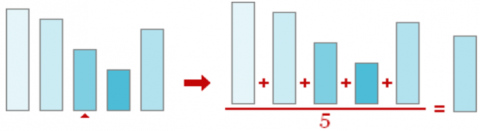
While for recording purposes we used PRAAT, ZOOMH1N digital speaker, and Online streaming editor. After recording the speech samples we applied preprocessing in order to remove the background noise. To remove the noise, we applied an average filter. The Average filter contains basic two steps.
1. A window should be placed over the feature.
2. Calculate average and replaced, the missing part by mean of all the sample values. The working of Average filter as shown below Figure 2 and Figure 3.
Table 1. Complete dataset description
|
S.NO |
Dialect |
Total time of speech data |
Speakers for each dialect |
Age of speakers |
Sampling Frequency |
|
1 |
Telangana |
2h 35 min |
22 |
20-55 |
44,100Hz |
|
2 |
Coastal Andhra |
2h 47 min |
19 |
20-55 |
44,100Hz |
|
3 |
Rayalaseema |
1h 43 min |
18 |
20-55 |
44,100Hz |
Figure 1. Basic structure followed to create the database
Figure 2. A Window (size of 5)
Figure 3. Calculation of average
After that, we are stored the data according to the dialects it belongs to. The complete statistics that we are used in the creation of the database as shown in Table 2.
Table 2. Different parameters used in database creation
|
Tools used for recording and editing |
PRAAT tool, Zoom H1N Handy Portable Digital Recorder, Streaming Audio Recorder |
|
Speakers age |
20 to 55 |
|
Number of dialects |
3 |
|
Number of speakers in each dialect |
Telangana (32), Kostha Andhra (27) Rayalaseema (23) |
|
Sample rate |
44kHz |
|
Channels |
MONO |
From the above table, it is observed that we are considered the different age speakers from 20 to 55 age group peoples to create the database and the sampling rate used is 44kHz.The number of speakers selected for the creation of the database varies from dialect to dialect. Telangana 32 peoples, Kostha Andhra 27 and Rayalaseema 23 speakers.
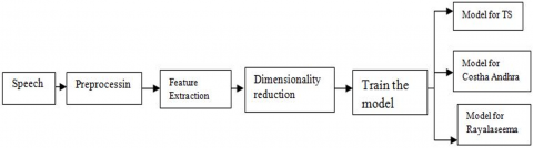
In order to identify the dialects of the Telugu Language, there are two stages are in methodology i.e., Training and Testing phase as described in Figure 4 and Figure 5.
4.1 Training
We collected the speech from the different users, considered it as input, then the speech is submitted to the preprocessing phase to reduce the background noise if it is present. For that, we used the average filter. The average filter provides smoothening and removes the variations (noise) and unvoiced parts. After completion of preprocessing submitted to Feature extraction. Now we extract the MFCC, ΔMFCC, ΔΔMFCC, and ZCR features from speech signals. After this phase, we combined these features, get 40 features of each sample i.e., 13 from MFCC, 13 from ΔMFCC, 13 from ΔΔMFCC, and 1 from ZCR. If we pass the same features for training, we may get up to lacks features approximately for the complete dataset, further, it will increase the burden of the model and time-consuming process. So, in order to reduce the number of features, we apply dimensionality reduction on those extracted features. In dimensionality reduction, we used the PCA method to reduce the number of features. PCA produces 30 features while eliminating less correlated features. After dimensionality reduction, we apply GMM and HMM models on the features. On applying these features, we frame out the models for Telangana, Costha Andhra, and Rayalaseema.
4.2 Testing
In the training, our models are made ready for different dialects. Now we test the models. We collect the speech sample from the user which we are going to test. The sample is preprocessed, and the unwanted noisy signal is eliminated using the average filter. Now we extract the 40 features i.e., MFCC, ΔMFCC, ΔΔMFCC, and ZCR. We reduce the number of features using PCA. Later we apply these features to the models and calculated the likelihood score. These scores are represented as Telangana are considered as β1, Costal Andhra as β2, Rayalaseema as β3. Then we compare β1, β2, β3. The highest among them is considered as the dialect of the speech sample.
Figure 4. Training model of the Telugu dialect identification
Figure 5. Testing phase of dialect identification
4.3 Proposed methods
For the identification of Telugu dialects, we used two classification models i.e., GMM and HMM models.
4.3.1 Hidden Markov Model
Hidden Markov Model (HMM) is a probabilistic graphical model that enables us to predict the sequence of the hidden or unknown variables from a set of observed variables. In this HMM (hidden Markov model), we do not know the actual probabilities of the variables, we only know their respective outcomes. The working of HMM model as shown below.
The basic structure of HMM model as shown in the following Figure 6.
Figure 6. Basic model of HMM
The HMM model contains the number of hidden states X1, X2….Xn and also Observable states y1,y2…..ym. It also contains different types of probabilities like transition probability a11, a12…anm, and also observation probability b11,b12…bxy. The complete description of HMM is
S=s1, s2….sN Number of hidden states.
O=o1,o2….oT, Number of observable sequence.
A= a11,a12,a13..a1n…ann, is transition probability matrix where aij represents the probability moving from state i to state j. Then all the moves corresponding to aij are equal to 1.
B=b1, b2…bn is the emission probability.
$\Pi$= π1 π2 π3… πn. represents the initial probabilities.
$\Pi$1 represents the probability to start initially from satae1. If π2=0 is indicating that state2 is not initial state. In our experiments, we have three hidden states i.e., Telangana, Costa Andhra and Rayalaseema. And we are used spectral and prosodic features like MFCC, PITCH and Loudness as observable states. So, there is 3 hidden states and 3 observables state, so T= 33=27 possible observations are occurred. To, find out the state of the event, calculate maximum likelihood. This will calculate by using the joint probability as shown below:
$P(O, Q)=P(O \mid Q) \times P(Q)=\prod_{i=1}^{T} P\left(o_{i} \mid q_{i}\right) \times \prod_{i=1}^{T} P\left(q_{i} \mid q_{i-1}\right)$
In the above equation can be explained like:
P (MFCC, PITCH, LOUDNESS, TS, CA, RS) = P(MFCC/TS) *P(PITCH/CA) *P(LOUDNESS/RS) *λ
λ = P(TS)*P(CA/TS) *P(RS/CA)
where, P(S) will not depend on any previous state we considered it as initial probability and remaining part of λ, indicates the transition probabilities and the first part is emission probabilities of states.
To understand HMM, let us consider predicting the weather based on the type of clothes that someone wears. Here weather acts as a hidden variable and the types of clothes are observed. Basically, the hidden Markov model is a Markov chain whose internal state cannot be explicitly observed, but the internal state of the model is used by the probabilistic function to evaluate only the probability distribution of the variables observed. HMM is mostly used in speech processing because,
• HMM is fabulously rich in mathematical structure and that is the reason it can form the theoretical basis for broad use in a wide range of applications.
• HMM model, when applied to the applications it works well practically in various important applications.
4.3.2 Gaussian Mixture Model
A Gaussian Mixture Model (GMM) is a density function of parametric probability, represented as a weighted sum of Gaussian component densities. Using the iterative Expect-Maximization (EM) algorithm or Maximum A Posteriori (MAP), estimate the GMM parameters. Which are works on training data. It is mainly used in biometric system where used to identify and authenticate the region of the user on the basis of his/her voice. In order to train audio files to recognize the spoken word, Gaussian Mixture Model is used. Gaussian Mixture Model tries to fix out the optimal values of these parameters to best fit our existing data. Mathematical Description of GMM.
p(x)=w1p1(x)+w2p2(x)+w3p3(x)+……. +wn pn(x)
where, p(x) = mixture component.
$w_{1}, w_{2}, \ldots w_{n}$= mixture weight or mixture coefficient.
$p_{i}(x)$= density functions.
The use of mixture components in GMM is to identify the number of cluster or components that where the data is going to fit. Each cluster or component contains the weights that indicates the probability that particular data point belongs to cluster.
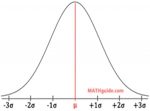
Figure 7. Bell curve
Bell Curve as shown Figure 7 is the probability density function of the Gaussian (normal) distribution.
µ = center of the distribution.
σ = Which tells us how the distribution is spread out.
$p(x)=w_{1} N\left(x \mid \mu_{1} \sum_{1}\right)+w_{1} N\left(x \mid \mu_{2} \sum_{2}\right)+\cdots+w_{1} N\left(x \mid \mu_{n} \sum_{n}\right)$
µ’s are means ∑’s is covariance-matrix of individual components.
In this, we have extracted the different spectral features like MFCC and its flavors and the temporal features like ZCR, which are extracted to identify the dialects. We also propose the combination of the features to identify the dialects.
5.1 Mel-frequency cepstral coefficients (MFCC)
Feature extraction is an especially important step in any speech recognition system. In order to find out the required components, extract the required features. In the sound production system, depends upon the shape of the vocal track sound pronunciation is varying. If we find the shape of the vocal track, we can exactly identify the required component. In order to find out the shape of the vocal track, we used MFCC features.
MFCC features are introduced in 1980. From the beginning onwards these features are widely used in all speech-related applications.
Steps involved in MFCC feature extraction:
1. Consider the speech signal s input and divide the speech signal into the number of frames.
2. calculate the power spectrum of each frame.
3. Add the energy of filters which is generated by the Mel filter bank.
4. Apply the logarithm to all energies.
5.Calculate DCT of energy.
These DCT coefficients are considered as MFCC features. For each frame extract, the 13 features and the remaining features are discarded.
The basic structure of extracting MFCC features as shown in the following Figure 8.
PSEUDOCODE FOR MFCC CALCULATION
Algorithm: MFCC feature extraction Pseudocode
Input: Pre-processed Speech signal
Output: Feature vector of MFCC
Function_MFCC (Pre-processed Speech signal):
Divide the signal into frames of size 5- 10 ms each one;
Apply the Hamming windowing technique to frames;
Apply FFT to covert time domain to frequency domain;
Calculate the Mel-filter bank;
Translate the frequency spectrum to mel spectrum;
Find the MFCC vectors for individual frames by applying DCT.
End Function_MFCC.
The signal is quasi in nature means it continuously changing in nature. In order to find out the required features, we are diving the speech into several frames each one has the size 5 to 10ms. After that depends upon cochlea in our production system frequency is presented in the signal. To extract that frequency, we used a periodogram. But thesis periodogram also extracts unnecessary features to ASR. in order to find out the required features we will use mel filter bank. if the frequency is high in speech filter banks are wider in the shape. How much space filter banks are spread we can find by using mel scale. After calculation of filter energies, take the algorithms of these energies, it is the normalization of channel technique. The louder voice is not possible to represent and extract the information after that calculate the DCT of log energies because frames that we divided in staring are overlapping to reduce the change of the features. DCT will decorrelate the energies up to a max of 13 features by using the following equation.
$c(n)=\sum_{M=1}^{M-1} \log 10(s(m)) \cos \left(\frac{\pi n(m-0.5)}{M}\right)$
where, n=0,1,2,…C-1
where, C id the number of MFCC features and oth feture always ignore because it indicates average log energy of the speech signal.
Figure 8. MFCC Feature extraction
Delta MFCC features can be extracted by taking the first derivative of MFCC features.
∆k=fk-fk-1
Delta Delta MFCC can be obtained by performing the derivative to Delta features.
∆∆k=∆k-∆k-1
In this research we are calculating 13 MFCC, 13 Delta MFCC and 13 Delta MFCC Features and applied to GMM and HMM models for identifying the dialects of Telugu language. The accuracies we got after applying to GMM and HMM as shown in the Table 3 and Table 4.
Table 3. Accuracies obtained by GMM with different feature extraction techniques
|
Model |
Feature Extraction Techniques |
Accuracy |
|
GMM |
MFCC |
70.2 |
|
MFCC+∆MFCC |
81.6 |
|
|
MFCC+∆MFCC+∆∆MFCC |
82.6 |
|
|
ZCR |
63.3 |
|
|
MFCC+∆MFCC+∆∆MFCC+ZCR |
83.3 |
Table 4. HMM accuracies with different feature extraction methods
|
Model |
Feature Extraction Techniques |
Accuracy |
|
HMM |
MFCC |
72.2 |
|
MFCC+∆MFCC |
73.833 |
|
|
MFCC+∆MFCC+∆∆MFCC |
82.6 |
|
|
ZCR |
73.33 |
|
|
MFCC+∆MFCC+∆∆MFCC+ZCR |
81.66 |
5.2 Zero-crossing rate
The zero-crossing (ZCR) is the rate at which a signal transitions from positive to negative to zero or from negative to positive to zero. In both speech recognition and music information retrieval, the importance of the zero-crossing rate has been commonly used and becoming a crucial function for classifying percussive sounds.
In order to separate the speech signal as voiced and unvoiced, we used generally ZCR and energy. The ZCR value is high for the unvoiced part and low for the voiced part. But the Energy is working is opposite to ZCR i.e. high foe voiced part and low for the unvoiced part. These two provides a good indication to separate the voiced and unvoiced part from the speech signal. The basic zero crossing of a signal as shown in Figure 9.
Figure 9. Zero crossings indication
In each interval of time, the zero-crossing rate is determined as the estimate of the number of times the amplitude of the speech signals passes through a value of zero.
Mathematical Description of Zero-crossing rate:
$Z_{\mathrm{n}}=\sum_{m=-\infty}^{\infty}|\operatorname{sgn}[x(m)]-\operatorname{sgn}[x(m-1)]| w(n-m)$
where,
$\operatorname{sgn}[\mathrm{x}(\mathrm{n})]=\left\{\begin{array}{c}1, x(n) \geq 0 \\ -1, x(n)<0\end{array}\right.$ and $\mathrm{w}(\mathrm{n})=\left\{\begin{array}{c}\frac{1}{2 N} \text { for } 0 \leq n \leq N-1 \\ 0, \text { otherwise }\end{array}\right.$
5.3 Principal component analysis
When the data contains a greater number of variables, it is difficult to analyze the data. It will increase the time of models to analyze. In order to reduce the attributes or variables and increase the efficiency of the model, better to reduce the unnecessary variables and find the required and more usable attributes. In order to find the required, we use the PCA. PCA is used to reduce the number of dimensions correlated data and turn the data into uncorrelated data points. The data generated by PCA easy to analyze and visualize the data. Principle component analysis is required because without it, the model suffers from ‘Over fitting’ problem, it means the model gets confused because of many values of attributes in the. The principal components are basically perpendicular to each as shown in the Figure 10 with maximum variance of data points.
Figure 10. Basic PCA components
Algorithm to find the PCA.
1)Find the mean of each attribute given in dataset.
2)Subtract each value in the dataset with its mean to make the data pass through origin.
3)Calculate the covariance matrix to observe the variance when two variables travel together.
4)Find Eigen values and Eigen vectors of the Co-variance matrix.
5) Choose P Eigen vectors with high Eigen values will be the principal component.
6. Project the data points into P Eigen vectors to make.
Now, for n dimensions of data we get n Eigen vectors, choose P Eigen vectors where p<n and the dimensions will be reduced. The block diagram of PCA as shown in following Figure 11.
The main advantage of PCA it would enable us to provide smaller inputs to our recognition system, which is an essential feature of our approach because it speeds up the training process while maintaining high precision means to decrease the computation cost in the recognition process. Another advantage is there is lack of redundancy in data because we are calculating eigenvectors that are perpendicular to each other. Noise reduction since the maximal variance basis is used, and minor differences in the context are simply discarded. For that we are applied the PCA to get good accuracy in recognition of dialects.
Figure 11. Methodology to calculate PCA
5.4 Proposed optimal feature extraction
To find the dialects of the Telugu language, we used the spectral feature extraction technique i.e., MFCC, and its flavors. We extracted the 39 feature vectors from speech samples by using MFCC. In these, 13 features are MFCC and 13 features Delta MFCC and 13 features are Dealt-Delta MFCC features and applied them to the models. We also extracted temporal future extraction techniques i.e., ZCR feature from the Speech signals. To increase the accuracy, we combine the features MFCC 39 features and ZCR features. Total it is 40 feature vectors applied to GMM and HMM models. The accuracies are shown in the Table 5 and Table 6. To reduce the number of features we used to apply the PCA. When we applied the PCA the number of features finally we for 25 feature vector. These features are used, given to the GMM and HMM models to find the dialects. The basic structure of the proposed reduced feature is shown in the Figure 12.
Figure 12. Proposed feature extraction methodology
Overall we applied two different statistical models GMM and HMM models to identify the dialects of the Telugu language. In order to identify we extracted the Spectral i.e. MFCC and flavours and temporal features i.e. ZCR. In order to increase the accuracy of models applied PCA to reduce the number of features without changing the algorithm and compare the results. As we observed that with PCA there increase in the accuracy to compare with original features.
Table 5. GMM accuracy with PCA
|
Model |
Reduced features with PCA |
Accuracy |
|
GMM |
MFCC |
70.2 |
|
MFCC+∆MFCC |
81.6 |
|
|
MFCC+∆MFCC+∆∆MFCC |
86.6 |
|
|
ZCR |
65.686 |
|
|
MFCC+∆MFCC+∆∆MFCC+ZCR |
85 |
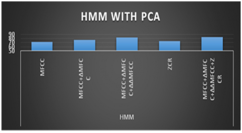
Table 6. HMM accuracies with PCA
|
Model |
Reduced features with PCA |
Accuracy |
|
HMM |
MFCC |
72.2 |
|
MFCC+∆MFCC |
76.66 |
|
|
MFCC+∆MFCC+∆∆MFCC |
82.6 |
|
|
ZCR |
73.3 |
|
|
MFCC+∆MFCC+∆∆MFCC+ZCR |
83.3 |
We applied different feature extraction techniques in order to identify the dialects. The following figures and tables show the results obtained by applying the GMM and HMM classification models.
From the above Table 3, it is observed that we applied the different types of MFCC features. In order to increase accuracy, we calculate the first and second differentiation of MFCC features. By applying the GMM model to MFCC+∆MFCC+∆∆MFCC features, it produces the results of 82.6%. When we apply the GMMM for ZCR it produces 63.3%. When we combine both features MFCC+∆MFCC+∆∆MFCC+ZCR then it provides good results 83.3%. The following Figure 13 shows the clear differentiation of accuracies.
Figure 13. Accuracies of GMM model with different feature extraction methods
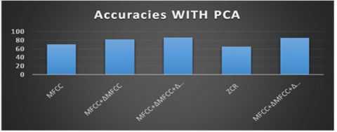
In order to increase the accuracy, we applied the Principal component analysis (PCA) to reduce the dimensionality of features. The Table 5 shows the accuracies produced by GMM when we applied the PCA to feature extraction techniques.
From the above table, it is observed that MFCC+∆MFCC+∆∆MFCC+ZCR features are applied to PCA to the reduced number of feature vectors. It produces 85 % accuracy with PCA. And without PCA it is 83.3%. The overall accuracy of the GMM model is increased when we applied to reduced features. The following Figure 14 shows the accuracy of the model with PCA.
The following Table 4 shows the accuracies of HMM model with different feature extraction techniques.
Figure 14. GMM accuracy with PCA
From the above table, HMM provides good results with MFCC+∆MFCC+∆∆MFCC features. It produced 81.66% with hybrid features MFCC+∆MFCC+∆∆MFCC+ZCR. The following Figure 15 shows the accuracy of the HMM model with different feature extraction techniques.
Figure 15. HMM accuracies without PCA
The above figure shows the accuracies of the HMM model without data reduction. From the above accuracies, it is observed that it produces good results for MFCC and its variations of features. The below Table 6, shows the accuracies of MFCC when we apply the data reduction techniques. It produced good results with Hybrid features. Means combine the features of MFCC and ZCR.
The following Figure 16 discriminate the accuracies of HMM model with PCA techniques.
Figure 16. HMM accuracies with reduction of features
The overall observation of Methods and different feature Extraction techniques, it is identified that the GMM model produced good results when the original features are reduced by PCA to identify the dialects. HMM, the model produces good results with original features of speech utterances. The following Table 7 describes the accuracies of models when we applied to original features and after reducing the features.
The following Figure 17, shows the clear difference of accuracies of models. HMM provides good results without applying the PCA and GMM provides good accuracy with PCA.
Table 7. Overall accuracies with and without PCA
|
Model |
without PCA |
WITH PCA |
|
GMM |
76.2 |
77.81 |
|
HMM |
76.71 |
77.6 |
Figure 17. Comparison of GMM and HMM model (with and without PCA)
Telugu dialects with optimized features are identified and to identify these dialects, MFCC, Delta MFCC and Delta Delta MFCC features are extracted along with ZCR features. Total 40 feature vectors are extracted for each speech sample. Dimensionality reduction techniques are applied to increase the efficiency and reduce the burden of the model i.e., PCA to reduce the number of features. After applying the PCA, the number of features is reduced from 40 to 30. After applying GMM and HMM model to identify the dialects, it is observed that without PCA, HMM model produced good accuracy with 76.71 compared to GMM it is 76.2. With PCA GMM provides good accuracy with 77.81 compared to HMM 77.6. In future, applying the deep learning models to increase the accuracy will enhance the results.
[1] Al-Walaie, M.A., Khan, M.B. (2017). Arabic dialects classification using text mining techniques. In 2017 International Conference on Computer and Applications (ICCA), pp. 325-329. https://doi.org/10.1109/COMAPP.2017.8079752
[2] Darjaa, S., Sabo, R., Trnka, M., Rusko, M., Múcsková, G. (2018). Automatic recognition of Slovak regional dialects. In 2018 World Symposium on Digital Intelligence for Systems and Machines (DISA), pp. 305-308. https://doi.org/10.1109/DISA.2018.8490639
[3] Shivaprsad, S., Sadanandam, M. (2020). Identification of regional dialects of Telugu language using text independent speech processing models. International Journal of Speech Technology, 23(1): 251-258. https://doi.org/10.1007/s10772-020-09678-y
[4] Al-Yami, R., Al-Zaidy, R. (2020). Arabic dialect identification in social media. In 2020 3rd International Conference on Computer Applications & Information Security (ICCAIS), pp. 1-2. https://doi.org/10.1109/ICCAIS48893.2020.9096847
[5] Leitner, C., Pernkopf, F. (2012). Speech enhancement using pre-image iterations. In 2012 IEEE International Conference on Acoustics, Speech and Signal Processing (ICASSP), pp. 4665-4668. https://doi.org/10.1109/ICASSP.2012.6288959
[6] Goswami, S., Deka, P., Bardoloi, B., Dutta, D., Sarma, D. (2013). A novel approach for design of a speech enhancement system using NLMS adaptive filter and ZCR based pattern identification. In 2013 1st International Conference on Emerging Trends and Applications in Computer Science, pp. 125-129. https://doi.org/10.1109/ICETACS.2013.6691408
[7] Trang, H., Loc, T.H., Nam, H.B.H. (2014). Proposed combination of PCA and MFCC feature extraction in speech recognition system. In 2014 International Conference on Advanced Technologies for Communications (ATC 2014), pp. 697-702. https://doi.org/10.1109/ATC.2014.7043477
[8] Kwon, O.W., Chan, K., Lee, T.W. (2003). Speech feature analysis using variational Bayesian PCA. IEEE Signal Processing Letters, 10(5): 137-140. https://doi.org/10.1109/LSP.2003.810017
[9] Abolhassani, A.H., Selouani, S.A., O'Shaughnessy, D. (2007). Speech enhancement using PCA and variance of the reconstruction error in distributed speech recognition. In 2007 IEEE Workshop on Automatic Speech Recognition & Understanding (ASRU), 19-23. https://doi.org/10.1109/ASRU.2007.4430077
[10] Ghosal, A., Chakraborty, R., Chakraborty, R., Haty, S., Dhara, B.C., Saha, S.K. (2009). Speech/music classification using occurrence pattern of zcr and ste. In 2009 Third International Symposium on Intelligent Information Technology Application, 3: 435-438. https://doi.org/10.1109/IITA.2009.427