Prasenjit Das* | Jay Kant Pratap Singh Yadav | Arun Kumar Yadav
© 2021 IIETA. This article is published by IIETA and is licensed under the CC BY 4.0 license (http://creativecommons.org/licenses/by/4.0/).
OPEN ACCESS
Tomato maturity classification is the process that classifies the tomatoes based on their maturity by its life cycle. It is green in color when it starts to grow; at its pre-ripening stage, it is Yellow, and when it is ripened, its color is Red. Thus, a tomato maturity classification task can be performed based on the color of tomatoes. Conventional skill-based methods cannot fulfill modern manufacturing management's precise selection criteria in the agriculture sector since they are time-consuming and have poor accuracy. The automatic feature extraction behavior of deep learning networks is most efficient in image classification and recognition tasks. Hence, this paper outlines an automated grading system for tomato maturity classification in terms of colors (Red, Green, Yellow) using the pre-trained network, namely 'AlexNet,' based on Transfer Learning. This study aims to formulate a low-cost solution with the best performance and accuracy for Tomato Maturity Grading. The results are gathered in terms of Accuracy, Loss curves, and confusion matrix. The results showed that the proposed model outperforms the other deep learning and the machine learning (ML) techniques used by researchers for tomato classification tasks in the last few years, obtaining 100% accuracy.
tomato maturity grading, manual grading, low-cost solution, AlexNet, deep learning, transfer learning
Tomatoes are one of the relevant crops for human taste. The protection and yielding in crop production can be improved using the proper and refined automation process. The country's economic growth can also be affected when applying intelligent cultivation methods in tomato production, as tomato is the major part of crops in most countries. Furthermore, a strong relationship exists between economic abundance and increases productivity. Therefore, the Tomato Maturity Grading system appears to be a potential way to overcome the significant problems of maintaining the quality of tomato production at lower production costs [1, 2].
The visualization of the tomato crop can be used to assess its maturity based on color, size, and shape. However, color is the most significant among these three categories. Therefore, the color of the tomato crop determined the time of product marketing since it profoundly impacts the customers' choice. Quality is the primary factor essential for efficient crop marketing. The primary predictor to evaluate the quality of vegetables and fruits like tomato is their maturity. Most potential customers evaluate the quality of fruit and vegetables through their physical or texture exhibition [3].
The conventional way of classifying Tomato Maturity is exceptionally exhausting and inaccurate. Moreover, overexertion and a heavy workload can affect human graders, which might harm the grading quality. It is a time-consuming process for organic farms. Manual Grading can also be different from person to person [4]. Therefore, automated maturity evaluation is a significant advantage to the agricultural sector. An automated Tomato Maturity Grading system may rule out anomalies in the maturity assessment through Manual Grading.
The automatic Tomato Maturity Grading system based on computer vision and machine learning approaches include mainly two different stages. The initial stage of the process involves the extraction of RGB color features. In the final stage, the tomato samples are classified based on their color features. Here, the proposed approach classified tomato maturity into three distinct classes: Red, Green, and Yellow.
Independent researchers and scholars have been developing an automated Tomato Maturity Grading system considering essential factors like color, size, shape, texture, etc. Conventionally, the majority of the Tomato Maturity Grading systems were developed using image processing techniques and machine learning.
Arjenaki et al. [5] introduced a machine vision-based approach to classifying the tomato samples into shape, size, maturity, and defects. The system achieved an accuracy of 89.4% for defect detection, 90.9%, and 94.5% accuracy for size and shape, respectively. The overall accuracy of the system is 90%. Arakeri et al. [6] designed a sorting system based on machine vision for defect detection of tomato samples. The accuracy of the sorting system is 96.47%. Liu et al. [7] classified the tomato samples into color, size, and shape. The proposed approach performed color-based classification by observing the range of hue values. First-Order-Fourier description(1D-FD) and a linear regression equation were used to classify the tomato samples into different shapes and sizes, respectively. The grading system achieved an average accuracy of 90.7%. Rokunuzzaman et al. [8], classified tomato defects (Blossom-End-Root and cracks) using color feature and shape. A new decision-based sorting method was introduced by combining a rule-based approach and neural networks. The accuracy of the system was found to be 84% for the rule-based approach and 87.5% for the neural network approach, respectively. Goel and Sehgal [9] developed a Fuzzy Rule-Based classification system (FRBCS) that used RGB color information to classify tomato maturity. The accuracy of the classification system is 94.29%. Opeña and Yusiong [10] extracted five color attributes: Red, Yellow, Red-Green, Hue, and a* from three color standards: RGB, HSI, and CIE L*a*b. The proposed system trained the Artificial Neural Network (ANN) classifier using Artificial Bee Colony (ABC0) algorithm. The classification technique achieved an accuracy of 98.19% using an ABC-trained ANN classifier. Pacheco and Lopez [11] utilized three-color standards: RGB, HIS, and L*a*b* to extract color features for data analysis. The proposed method applied three different classifiers: K-NN (K-Nearest Neighbors), MLP type Neural Networks (Multilayer Perceptron), and K-Means for Tomato Maturity Grading. The experimental results showed that the K-NN classifier incorporated with MLP neural network got the best performances compared to other techniques.
Recent progress in Deep Learning has created opportunities for new agricultural applications. Deep Learning has now been introduced as an excellent learning method in image classification, machine vision, and many others. A striking feature of Deep Learning techniques is automatic feature extraction, which helps to learn useful information from a massive image data set [12]. Moreover, Deep Learning improves our knowledge of human sensitivity, thus evolving the conventional machine learning approach. Liu et al. [13] introduced a tomato maturity detection system based on DenseNet deep neural network architecture. The proposed system works efficiently to detect tomato maturity even in a complex background. Zhang et al. [14] developed a tomato maturity classification system with better precision and reliability. They used a convolution neural network (CNN) to classify the maturity. The proposed system achieved an overall accuracy of 91.9% with a prediction time of lesser than 0.01 seconds. Brahimi et al. [15] introduced an automated plant disease classification system that classified 14,828 images of infected tomato leaves into nine distinct categories of diseases. The classification system managed to achieve the performance of identifying leaf diseases with up to 99.18% accuracy.
Recently, an automated classification system using CNN has made significant achievements in several challenges. The organized architecture and extensive range of learning competencies of CNN models make them pretty effective and versatile in terms of classification and prediction [16]. However, the Deep neural network (DNN) system sometimes faces overfitting problems, even though reliability in certain domains has been phenomenal. Overfitting problems occurred primarily due to three factors: complex structure of the model, data noise, and less training data set [14]. Moreover, generating a dataset including sufficient samples is sometimes challenging, and it takes too much time. Thus, data augmentation is an efficient way to increase input data artificially whenever there are limited data in the dataset.
This paper introduced an automated tomato grading system based on Convolution Neural Network using Transfer Learning. Transfer Learning permits different areas, exercises, and distributions for training and testing. This research aims to establish a color analysis approach to evaluate the color characteristics of market-fresh tomatoes and then classified the tomatoes based on three maturity stages: Red, Yellow, Green using Alexnet pre-trained network (Transfer Learning). The results are gathered in terms of Accuracy and loss curves, and confusion matrix. The results showed that the proposed model outperforms the other deep learning and the machine learning (ML) techniques used by researchers for tomato classification tasks in the last few years, obtaining 100% accuracy.
The remainder of the paper is organized as follows. Section 2 describes the materials and methods used to classify the Tomato Maturity Grading. Section 3 analyses experimental results and discussion. Finally, section 4 concludes the paper.
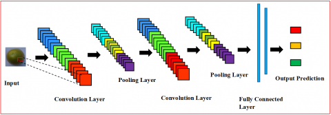
The classification system based on CNN can increase their performance and accuracy if there are sufficient data sets available for the problem. Typically, CNN comprises several layers, beginning with an input layer followed by hidden layers and terminating with an output layer. Basic CNN architecture has been shown in Figure 1. The input layer is just where the data is added into the network and works as an input for subsequent layers. Each hidden layer of CNN architecture includes distinct convolutional, pooling, and fully connected layers [17]. The convolution layer is used to extract valuable features automatically from the input dataset (for example, tomato image). The pooling layer minimized the dimension of those input image datasets, while classification is done by the fully connected layer [18]. Typically, the fully connected layers learned useful features and utilized those features to classify the input image dataset into pre-determined classes.
Figure 1 Basic CNN structure
2.1 Convolution layer
A convolution layer is the central unit of CNN architecture that handles the majority of the convolution process. Each convolution layer comprises convolutional filters(kernels) executed on the inputs to generate an output, sometimes named feature maps [19]. Suppose an input data D of dimension m x n with a kernel F of size p x q. The output R of this convolutional layer is given by a two-dimensional convolution,
$R(u, v)=\sum_{i, j} D(i, j) F(i-u, j-v)$ (1)
The convolution operation can be defined as sliding the filter from right to left and from top to bottom. Between the slides, the filter and input matrix is multiplied component-wise, and all of the components are integrated to generate a scalar output. The weight matrix elementary product (kernel or filter) and the image pixels are computed in the convolution process. It aims to obtain critical features such as the edges of an object from the input image.
2.1.1 Stride(S)
When S=1, the filter window is slide by 1 pixel accordingly. Likewise, more than one pixel can be used to slide the window. The sliding number of pixels is known as a stride. However, larger strides cause the receptive fields to overlap less with smaller feature maps as more positions are dropped out. Therefore, the feature map is reduced in size relative to the input.
2.1.2 Padding(P)
Padding is used to maintain the same dimension as the input by simply placing a few numbers of zero’s in the image boundary, also known as zero paddings. However, the additional zero compiled depends on the size of the selected convolution filter [20]. Therefore, if the selected filter size is 3, then the additional zeros compiled is 1 using the following formula,
No. of zero's added $=\left[\frac{F-1}{2}\right]$ (2)
where, F is the size of the filter.
The size of the receptive field and output matrix for the mapping features are calculated using these hyperparameters. The dimension of the receptive field can be calculated using the formula,
$R_{1}=\left(\frac{q-F_{0}+2 P_{0}}{S_{0}}\right)+1$ (3)
$R_{2}=\left(\frac{t-F_{1}+2 P_{1}}{S_{1}}\right)+1$ (4)
where, P denotes the padding of zeros or ones, $F_{0}$, $F_{1}$, $S_{0}$, and $S_{1}$ refer to filter width, filter height, stride width, and stride height, respectively.
The performance matrix for the pooling layer is calculated using the formula,
$R_{m}=\left(\frac{K_{m}-F+2 P}{S}\right)+1$ (5)
where, $R_{m}$ is represented as a performance matrix, $K_{m}$ represents the input matrix, P denotes the padding of zeros or ones, F represents the filter size, and S refers to the width or height of stride.
2.2 Activation functions
The convolution process results are exceeded by an activation function, which brings non-linearity to the network. Thus, Non-linearity increases the power of a neural network [21]. However, an activation function operates on each component of the input data. The rectified linear unit (ReLU) is an effective activation function for the training of deep neural network for the supervised task, mathematically represented as,
$R(y)=\max (0, y)$ (6)
It is much easier to measure and produce results using the ReLU function than the Sigmoid function that requires exponential calculations. The Sigmoid values can be computed as,
$S(x)=\frac{1}{\left(1+e^{-x}\right)}$ (7)
2.3 Pooling layer
It is a subsample/reduction layer that is normally applied after the activation layer. It significantly reduces the duplication in the input components and also monitors overfitting [20]. By default, a 2x2 filter is usually used as an input to generate output depending upon the form of pooling. However, max or average pooling are different forms of pooling, where the max or average value is taken from each subsection that is restricted by the filter.
2.4 Fully connected layer
A fully connected layer (also known as the dense layer) recognizes top-level features that are quite similar to a class or entity. The input to a fully connected layer is a group of attributes for the image classification ignoring the spatial structure of the image [22]. A fully connected layer obtains a vector p as input and generates another vector q as output, which can be represented mathematically by a matrix-vector multiplication:
$q=R p$ (8)
where, $p \in W^{n}$ and $R \in W^{m \times n}$ is a trainable weight matrix. The term “Fully connected” is based upon the fact that the output element is a weighted total of all input elements.
One significant belief across many Deep Learning and machine learning algorithms is that the training and future data must be in similar feature spaces and shared equally. Nevertheless, this hypothesis may not exist for many real-world applications. As the distribution alters, it is necessary to reconstruct the statistical model from scratch using newly collected training data. However, it is costly or impractical to re-group sufficient training data and reconstruct the models in specific real-world applications [23]. In such cases, Transfer Learning will significantly increase learning efficiency by eliminating expensive and complex data labeling efforts. In recent years, Transfer Learning has become a new methodology to resolve this issue. Here, we used pre-trained AlexNet based on the Convolution Neural Network as the basic Transfer Learning model for the classification of Tomato Maturity Grading. The general edition of AlexNet is pre-trained with the ImageNet15 data set, which includes more than 1 million images and around 1000 available classes [24]. The weights of the model are pre-determined by a pre-trained network rather than dynamically determine during training from scratch.
3.1 Data used
In this experiment, approximately 200 color images were obtained from the local market for each of the three maturity stages: Red, Yellow, Green. Maturity of color is taken based on the color matching of tomatoes from the tomato color chart given by the United States Department of Agriculture (USDA), which shows six stages of maturity: Red, Light Red, Pink, Turning, Breakers and Green. In this paper, the three stages have been made by merging the Red and Light red into Red, Pink, Turning, Breakers into Yellow, and green due to simplicity according to Indian cultivation. Some of the collected data samples are shown in Figure 2. Initially, around 250 images were captured as sample images data set of all three colors or classes.
The dataset contains the three classes of tomatoes classified based on color as:
Class 0: Red Tomato
Class 1: Yellow Tomato
Class 2: Green tomato
However, this was a pretty less number of images than what is usually required for Deep neural network training. Therefore, to expand the limited number of training samples, we applied augmentation with a dynamic rotation of 0°-360° [25]. Augmentation significantly increases the number of training samples (total 2999 images). To train the Softmax classifier, 70% of images are used as a training set, and the remaining 30% are used as a test set to test the performance of the model.
Figure 2. Sample images of tomato
3.2 Proposed methodology
In contrast to previous approaches, we introduced a Transfer Learning approach to classifying Tomato Maturity Grading. The fundamental task is to select a pre-trained network as a basic Transfer Learning model with a pretty complex structure and successfully trained from a large data source, namely ImageNet, the huge database used for the research on visually identifying objects. ImageNet includes 22,000 categories of objects.
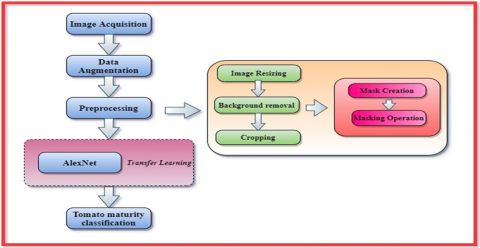
TL aims to transfer the knowledge acquired from a large data source (e.g., ImageNet) and enhance learning for a relevant assigned task [26, 27]. The benefits of TL as compared to the conventional Deep Learning approach in the context of real-world application are: (a) As a baseline, TL uses a pre-trained model. (b)Generally, it is easier and faster to calibrate a pre-trained model rather than to train a separate random Deep Learning model. Figure 3 illustrates the proposed structure for an automated Tomato Maturity Grading system using AlexNet as a basic Transfer Learning model.
Figure 3. The proposed framework for Tomato Maturity Grading using pre-trained AlexNet
3.2.1 Image acquisition
During the image acquisition process, we captured the tomato images under the normal fluorescent light sources using a color digital camera (Nikon D3500) with a resolution of 1920x1080 pixels and a lens zoom of between 18 and 55 mm. The tomato samples were collected from the nearby market. The tomatoes were placed on the surface of a clean white paper during the image capturing process to keep the background clear and take the tomato image clearer and noise-free due to color refractions. Images were captured during daylight hours to take a clear picture to avoid color blinding issues for the camera.
However, in a real-life scenario, other factors like the presence of any object between tomato and camera, presence of other objects during image capture, and so on may also occur. This paper only focuses on the performance of the proposed model in a simple scenario, but the aforementioned complex cases can also be considered in future works by applying other pre-processing steps to remove such types of noises from the captured image.
3.2.2 Data augmentation
The efficiency of deep convolution neural networks can be improved significantly by expanding the number of training samples [28]. Figure 4 shows the augmented image of the tomato sample.
Figure 4. Augmented image of tomato sample
Some of the data augmentation techniques usually involve: Flipping, Cropping, Shifting, PCA jittering, Color jittering, Noise, Rotation, etc.
3.2.3 Image pre-processing
After acquiring the tomato images in RGB, it is significantly important to apply pre-processing on tomato images to maintain color feature values accurately. In this experiment, the pre-processing techniques we applied are: resizing, background removal, and cropping.
Image resizing. Image resizing is the very first pre-processing technique. Throughout this experiment, the image resizing task is performed twice. Initially, the tomato images were resized with a dimension of 200 x 200 pixels before the background removal task. Thus, it helps to make the background removal task substantially faster and more efficient. Finally, the image resizing is performed for the second time with a dimension of 64 x 64 pixels after images have been cropped.
Background removal. Background removal process consist of four distinct steps:
Step 1: Blue channel transformation.
Step 2: Grayscale transformation.
Step 3: Creation of binary mask.
Step 4: Background removal using the binary mask.
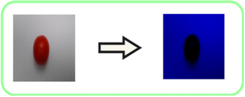
The background removal process starts with the blue channel transformation of an RGB image, as shown in Figure 5. The blue channel is itself a subset of the RGB model. Therefore, the blue channel transformation of an RGB image is carried out by simply assigning the values of red and green units to zero. Thus, only the blue unit holds its value, as illustrated in Figure 6.
Figure 5. An RGB image to blue channel transformation
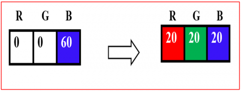
Figure 6. Blue channel transformation
The grayscale transformation process is the second step in the background removal task. During the grayscale transformation process, the blue channel image is transformed to a grayscale image by calculating the mean value as follows,
GrayScale $=\frac{(R+G+B)}{3}$ (9)
It is apparent from Figure 7 that each pixel in a grayscale image holds the same values for all three color units. Therefore, each pixel can be identified as a single value in a grayscale image. The conversion of an image from the blue scale to grayscale is illustrated in Figure 8.
Figure 7. Grayscale image transformation
Figure 8. A blue channel image to grayscale image transformation
Binary mask creation is the third step of the background removal task. In this paper, the binary mask is created using Otsu's method [29]. Nobuyuki Otsu developed Otsu's method, and it is a histogram-based binarization approach. Figure 9 shows the binary mask generated by applying the otsu’s method.
Figure 9. Creation of a binary mask
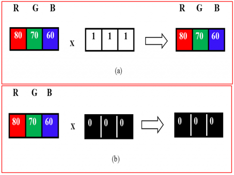
The last phase of background removal is to apply the binary mask to the colored image. As is shown in Figure 10(c), the region of interest is obtained from a colored image through the multiplication of the colored image and the binary mask. As is shown in Figure 10(a), when the binary mask’s pixel value is 1, the item is identical to the actual pixel. Nevertheless, when the pixel value of the binary mask is 0, the item is identical to the binary mask pixel, as shown in Figure 10(b).
Figure 10. The masking operation
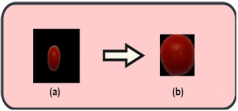
Image cropping. There is no need for background pixels in the feature extraction stage. Therefore, to optimize the processing time, the background pixels should be removed. In this paper, the image cropping task is performed to minimize these background pixel. The background pixels are illustrated by black color, as shown in Figure 11(a), and the cropped image of the tomato sample is shown in Figure 11(b).
3.2.4 AlexNet (Transfer Learning)
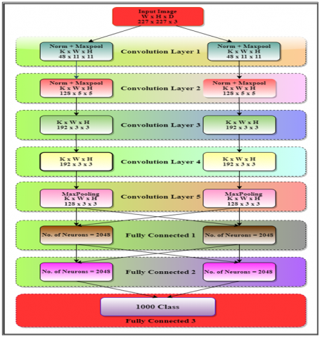
AlexNet ranked the first position in the ImageNet competition, which was held in 2012, obtained a top-5 error of just 15.3%, and acquired 10.8% higher than the performance of runner-up who utilized a shallow neural network [30]. Typically, AlexNet was operated using two graphics processing units (GPUs). Currently, experts are using only a single GPU for the implementation of AlexNet. This research incorporates only layers with learnable weights. Therefore, AlexNet comprises a total of 8 layers, five convolution layers (CLs), and three fully connected layers (FCLs). Figure 12 shows the AlexNet Architecture.
Figure 11. Image cropping
Figure 12. Architecture of AlexNet
In this study, we used a pre-trained CNN model to classify different maturity stages of tomatoes. Hence, we have to optimize the last three layers of the original AlexNet architecture. Throughout the optimization task, the top k layers of the original AlexNet model are fixed, and the rest of the (n-k) layers are customized. Table 1 details the layers of AlexNet, including activations and learnable weights.
As the size of output neurons of conventional AlexNet (around 1000 classes) is not the same as the number of classes in our proposed system (3 classes: Red, Yellow, Green), therefore it is necessary to modify the identical softmax layer and classification layer. Table 2 shows the modification of AlexNet. Thus, in our Transfer Learning strategy, we adopted a newly customized fully connected layer of three neurons, a softmax layer, and a classification layer of only three classes (Red, Yellow, Green). Table 3 details the hyperparameter values used during the entire training process of AlexNet.
Table 1. Detail analysis of AlexNet
|
Name |
Type |
Activations |
Learnables |
|
data |
Image Input |
227x227x3 |
- |
|
conv1 |
Convolution |
55x55x96 |
Weights 11x11x3x96 Bias 1x1x96 |
|
pool 1 |
Max Pooling |
27x27x96 |
- |
|
conv2 |
Grouped Convolution |
27x27x256 |
Weights 5x5x48x128x2 Bias 1x1x128x2 |
|
pool2 |
Max Pooling |
13x13x256 |
- |
|
conv3 |
Convolution |
13x13x384 |
Weights 3x3x256x384 Bias 1x1x384 |
|
conv4 |
Grouped Convolution |
13x13x384 |
Weights 3x3x192x192x2 Bias 1x1x192x2 |
|
conv5 |
Grouped Convolution |
13x13x256 |
Weights 3x3x192x128x2 Bias 1x1x128x2 |
|
pool5 |
Max Pooling |
6x6x256 |
- |
|
fc6 |
Fully Connected |
1x1x4096 |
Weights 4096x9216 Bias 4096x1 |
|
fc7 |
Fully Connected |
1x1x4096 |
Weights 4096x4096 Bias 4096x1 |
|
fc8 |
Fully Connected |
1x1x1000 |
Weights 1000x4096 Bias 1000x1 |
|
prob |
Softmax |
1x1x1000 |
- |
|
output |
Classification Output |
- |
- |
Table 2. Modification of AlexNet
|
Layer No. |
Original Layer |
Customized |
|
23. |
fc8 (1000 fully connected layer) |
fc8 (3fully connected layer) |
|
24. |
Prob (Softmax Layer) |
Softmax Layer |
|
25. |
Classification Layer (1000 classes) |
Classification Layer (3 classes: Red, Yellow, Green) |
Table 3. Hyperparameter values of AlexNet
|
1. |
Optimization Scheme |
SGDM (Stochastic Gradient Descent with Momentum) |
|
2. |
Minimum learning rate |
0.0001 |
|
3. |
Minimum Batch Size |
10 |
|
4. |
Max Epochs |
6 |
|
5. |
Validation Frequency
|
3 |
|
6. |
Momentum |
0.9 |
|
7. |
Dropout Rate |
0.5 |
3.2.5 Tomato maturity classification
Classifiers can be either binary or multi-class classifiers. The sigmoid activation function is used to solve binary classification problems, while the softmax regression is used to classify multi-class problems. In this paper, the classification of the tomato samples into three distinct classes: Red, Yellow, and Green, is performed using the Softmax function. It follows a probability distribution in the range (0,1), and output sums up to 1. The softmax function can be mathematically represented as,
$F(x): Q^{N} \rightarrow Q^{N}$ (10)
where an individual component of this specific vector can be calculated as,
$F_{z}=\frac{e^{x_{z}}}{\sum_{j=1}^{T} e^{x_{j}}} \forall z \in 1 \ldots N$ (11)
where, $F_{z}$ is invariably positive within range value (0,1), since the numerator together with the other summation values occurs in the denominator. Such characteristics allow itself suitable for the predictive analysis of a specified input class. The softmax function can be calculated as follows,
$F_{z}=K(f=z \backslash x)$ (12)
where, f represents the specified output class from (1 ... N) for N-dimensional vector x, regarding the classification of each multiclass problem.
The experiments are tested on a PC equipped with a 1.80GHz, Intel® quad-Core i5-8265U CPU processor in order to enable the parallel processing to enhance the computation power of classification task, 250 GB SSD, and 8GB RAM. The software application used to analyze the data is Matlab 2019b.
Before training, three particular were optimized. First, for Transfer Learning, the entire training epoch must be minimal. Hence, the training epoch number is adjusted to 6. Furthermore, the global learning rate is adjusted to a minimum rate of 0.0001 to decelerate the training process since the initial neural network layers were pre-trained. Third, we adjusted a 10-fold training rate for new layers, as their weights were customized randomly rather than pre-trained.
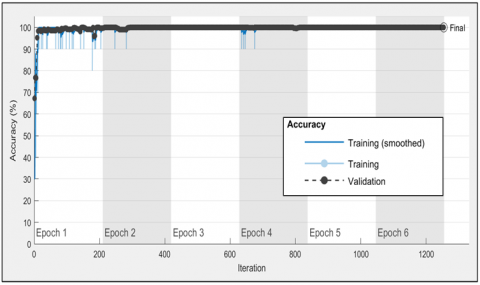
Figure 13. Training and validation results of AlexNet.
The fine-tuned AlexNet is trained using 700 tomato images of each class. However, the training is carried out using a single GPU. Hence, to inhibit limited memory lapses and maximize the learning process, we set the minimum batch size to 10. Though, the training terminated following 1254 iterations as the accuracy of the validation is balanced.
Here, Gradient Descent with Momentum (SGDM), the momentum of 0.9, has been used as the primary training function. The results of the training and testing are shown in Figure 13. Initially, the training process was unbalanced because of the small minimum batch size. However, using 300 images for each training epoch significantly increases the validation accuracy. Figure 14 shows the loss rate of AlexNet.
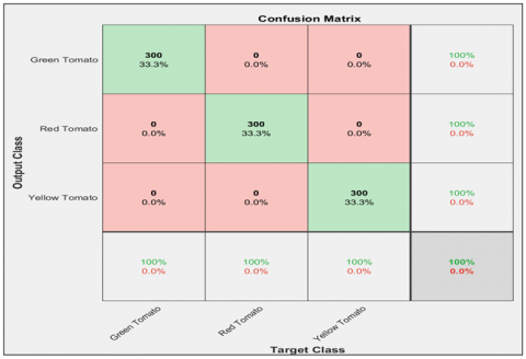
Validation operation is performed using 900 images, and Figure 15 shows the confusion matrix. The experimental analysis shows all three pre-determined classes are successfully identified, and our proposed approach managed to achieve an overall accuracy of 100%, as verified by Figure 13.
Figure 14. The loss rate of AlexNet
Figure 15. Validation results of AlexNet
The performance of the AlexNet classifier can be calculated as follows,
Accuracy $=\frac{\text { No. of correctly classified images }}{\text { Total number of images }}$
$=\frac{300+300+300}{600}=\frac{900}{900}=100$ (13)
This proposed Transfer Learning approach was compared with three state-of-the-art approaches: Fuzzy Rule-Based Classification approach (FRBCS), ABC-trained ANN Tomato Classification approach, First-Order-Fourier description(1D-FD) approach. Table 4 and Figure 16 show the comparison results of the proposed approach (AlexNet) with other existing approaches.
Table 4 and Figure 16 show that the proposed Transfer Learning approach had the highest accuracy than other traditional state-of-the-art approaches. Hence, the proposed Transfer Learning approach based AlexNet classifier is efficient and could be used for the tomato maturity classification.
Table 4. Comparison of the proposed approach with other existing approaches
|
Author |
Year |
Approaches |
Overall Accuracy (%) |
|
Goel et al. [9] |
2015 |
Fuzzy Rule-Based Classification approach (FRBCS) |
94.29% |
|
Opena et al. [10] |
2017 |
ABC-trained ANN Tomato Classifier |
98.19 % |
|
Liu et al. [7] |
2019 |
First-Order-Fourier description(1D-FD) |
90.7% |
|
Our proposed Approach |
2020 |
Finetuned AlexNet |
100% |
Figure 16. Performance comparison graph
This paper introduced a Transfer Learning approach and utilized it to develop an automated Tomato Maturity Grading system. the proposed method used a well-performed pre-trained CNN model, namely AlexNet, to take advantage of the Transfer Learning. Transfer learning applied at the last three layers to customize the AlexNet as per our proposed method's requirement. Hence Alexnet is customized with a fully connected layer of three neurons, a softmax layer, and a classification layer of only three classes to classify tomato images into three distinct maturity stages: Red, Yellow, and Green, based on their color feature analysis. The dataset was prepared using the augmentation process applied on the camera captured tomato images from a local market. The augmentation process increased the number of images in the dataset that prevented the model from overfitting issues during training with fewer image samples captured. The experimental results showed that the proposed method achieved promising results with an overall accuracy of 100%. Our proposed method has less computation of parameters and better precision as compared to other available standard architecture. As an application, this model can be used efficiently in the maturity classification of tomatoes which are to be kept in a clean environment and, based on their maturity, are used for different purposes like the most matured (red) tomato can be used for making tomato ketchup, and less matured (green) tomato can be kept further till its perfect maturity.
However, we should also keep in mind that using a pre-trained CNN limits us from using its existing architecture. Therefore, our data had to be adapted to an architecture that is fair sub-optimal for tomato images. Although it is possible to modify the input images and select the output layers, our capability to customize the existing architecture of AlexNet is minimal.
The approach used in this paper can precisely identify the maturity stages of tomato images. However, the model performs slowly due to many calculations generated by the Deep Learning model. Future work includes implementing a lightweight Deep Learning model from scratch, specifically trained to classify the maturity stages of tomatoes.
[1] Sembiring, A., Budiman, A., Lestari, Y.D. (2017). Design and control of agricultural robot for tomato plants treatment and harvesting. Journal of Physics: Conference Series, 930: 012019. https://doi.org/10.1088/1742-6596/930/1/012019
[2] Wang, L.L., Zhao, B., Fan, J.W., Hu, X.A., Wei, S., Li, Y.S., Zhou, Q.B., Wei, C.F. (2017). Development of a tomato harvesting robot used in greenhouse. International Journal of Agricultural and Biological Engineering, 10(4): 140-149. https://doi.org/10.25165/j.ijabe.20171004.3204
[3] Villaseñor-Aguilar, M.J., Botello-Álvarez, J.E., Pérez-Pinal, F.J., Cano-Lara, M., León-Galván, M.F., Bravo-Sánchez, M.G., Barranco-Gutierrez, A.I. (2019). Fuzzy classification of the maturity of the tomato using a vision system. Journal of Sensors, 2019: 1-12. https://doi.org/10.1155/2019/3175848
[4] Syahrir, W.M., Suryanti, A., Connsynn, C. (2009). Color grading in Tomato Maturity Estimator using image processing technique. 2009 2nd IEEE International Conference on Computer Science and Information Technology. https://doi.org/10.1109/iccsit.2009.5234497
[5] Arjenaki, O.O., Moghaddam, P.A., Motlagh, A.M. (2013). Online tomato sorting based on shape, maturity, size, and surface defects using machine vision. Turkish J. Agric. Forest, 37: 62-68. http://dx.doi.org/10.3906/tar-1201-10.
[6] Arakeri, M., Lakshmana. (2016). Computer vision based fruit grading system for quality evaluation of tomato in agriculture industry. Procedia Computer Science, 79: 426-433. https://doi.org/10.1016/j.procs.2016.03.055
[7] Liu, L., Li, Z., Lan, Y., Shi, Y., Cui, Y. (2019). Design of a tomato classifier based on machine vision. PLOS ONE, 14(7): e0219803. https://doi.org/10.1371/journal.pone.0219803
[8] Rokunuzzaman, M., Jayasuriya, H. (2013). Development of a low cost machine vision system for sorting of tomatoes. Agric Eng Int: CIGR Journal, 15(1).
[9] Goel, N., Sehgal, P. (2015). Fuzzy classification of pre-harvest tomatoes for ripeness estimation – An approach based on automatic rule learning using decision tree. Applied Soft Computing, 36: 45-56. https://doi.org/10.1016/j.asoc.2015.07.009
[10] Opeña, H.J.G., Yusiong, J.P.T. (2017). Automated tomato maturity grading using ABC-trained artificial neural networks. Malaysian Journal of Computer Science, 30(1): 12-26. https://doi.org/10.22452/mjcs.vol30no1.2
[11] Pacheco, W.D.N., Lopez, F.R.J. (2019). Tomato classification according to organoleptic maturity (coloration) using machine learning algorithms K-NN, MLP, and K-Means Clustering. 2019 XXII Symposium on Image, Signal Processing and Artificial Vision (STSIVA). https://doi.org/10.1109/stsiva.2019.8730232
[12] Zhu, L., Li, Z., Li, C., Wu, J., Yue, J. (2018). High performance vegetable classification from images based on AlexNet Deep Learning model. International Journal of Agricultural and Biological Engineering, 11(4): 190-196. https://doi.org/10.25165/j.ijabe.20181104.2690
[13] Liu, J., Pi, J., Xia, L. (2019). A novel and high precision tomato maturity recognition algorithm based on multi-level deep residual network. Multimedia Tools and Applications. https://doi.org/10.1007/s11042-019-7648-7
[14] Zhang, L., Jia, J., Gui, G., Hao, X., Gao, W., Wang, M. (2018). Deep learning based improved classification system for designing tomato harvesting robot. IEEE Access, 6: 67940-67950. https://doi.org/10.1109/access.2018.2879324
[15] Brahimi, M., Boukhalfa, K., Moussaoui, A. (2017). Deep learning for tomato diseases: Classification and symptoms visualization. Applied Artificial Intelligence, 31(4): 299-315. https://doi.org/10.1080/08839514.2017.1315516
[16] Oquab, M., Bottou, L., Laptev, I., Sivic, J. (2014). Learning and transferring mid-level image representations using convolutional neural networks. 2014 IEEE Conference on Computer Vision and Pattern Recognition. https://doi.org/10.1109/cvpr.2014.222
[17] Canziani, A., Paszke, A., Culurciello, E. (2017). An analysis of deep neural network models for practical applications. ArXiv, abs/1605.07678
[18] Schmidhuber, J. (2015). Deep learning in neural networks: An overview. Neural Networks, 61: 85-117. https://doi.org/10.1016/j.neunet.2014.09.003
[19] Goodfellow, I., Bengio, Y., Courville, A., Bengio, Y. (2016). Deep Learning. MIT Press Cambridge.
[20] Francis, M., Deisy, C. (2019). Disease detection and classification in agricultural plants using convolutional neural networks – A visual understanding. 2019 6th International Conference on Signal Processing and Integrated Networks (SPIN). https://doi.org/10.1109/spin.2019.8711701
[21] Saini, G., Khamparia, A., Luhach, A.K. (2019). Classification of plants using convolutional neural network. First International Conference on Sustainable Technologies for Computational Intelligence Advances in Intelligent Systems and Computing, pp. 551-561. https://doi.org/10.1007/978-981-15-0029-9_44
[22] Jassmann, T.J., Tashakkori, R., Parry, R.M. (2015). Leaf classification utilizing a convolutional neural network. Southeast Con. https://doi.org/10.1109/secon.2015.7132978
[23] Pan, S.J., Yang, Q. (2010). A survey on transfer learning. IEEE Transactions on Knowledge and Data Engineering, 22(10): 1345-1359. https://doi.org/10.1109/tkde.2009.191
[24] Huynh, B.Q., Li, H., Giger, M.L. (2016). Digital mammographic tumor classification using Transfer Learning from deep convolutional neural networks. Journal of Medical Imaging, 3(3): 034501. https://doi.org/10.1117/1.jmi.3.3.034501
[25] Liu, G., Mao, S., Kim, J.H. (2019). A mature-tomato detection algorithm using machine learning and color analysis. Sensors, 19(9): 2023. https://doi.org/10.3390/s19092023
[26] Soudani, A., Barhoumi, W. (2019). An image-based segmentation recommender using crowdsourcing and Transfer Learning for skin lesion extraction. Expert Systems with Applications, 118: 400-410. https://doi.org/10.1016/j.eswa.2018.10.029
[27] Wang, S.H., Xie, S., Chen, X., Guttery, D.S., Tang, C., Sun, J., Zhang, Y.D. (2019). Alcoholism identification based on an alexnet transfer learning model. Frontiers in Psychiatry, 10. https://doi.org/10.3389/fpsyt.2019.00205
[28] Jia, S.J., Wang, P., Jia, P.Y., Hu, S.P. (2017). Research on data augmentation for image classification based on convolution neural networks. 2017 Chinese Automation Congress (CAC). https://doi.org/10.1109/cac.2017.8243510
[29] Otsu, N. (1979). A threshold selection method from gray-level histograms. IEEE Transactions on Systems, Man, and Cybernetics, 9(1): 62-66. https://doi.org/10.1109/tsmc.1979.4310076
[30] Krizhevsky, A., Sutskever, I., Hinton, G.E. (2017). ImageNet classification with deep convolutional neural networks. Communications of the ACM, 60(6): 84-90. https://doi.org/10.1145/3065386