Yonghong Tian* | Bing Zheng | Zeyu Li | Yue Zhang | Qi Wu
© 2020 IIETA. This article is published by IIETA and is licensed under the CC BY 4.0 license (http://creativecommons.org/licenses/by/4.0/).
OPEN ACCESS
In the Internet age, online car hailing (OCH) platforms are increasingly popular among travelers. The efficiency of the OCH platform relies on the accurate forecast of OCH supply-demand. This paper attempts to forecast the OCH supply-demand accurately in each area of the target city based on deep learning (DL). Firstly, the authors introduced the structures of the long short-term memory (LSTM) and its variants, and established a single-gate model called minimal coupled LSTM (MC-LSTM). To improve the forecast effect, the MC-LSTEM was trained by the Nesterov-accelerated adaptive moment estimation (Nadam) algorithm. After that, the features that affect the OCH supply-demand forecast were identified. Based on the features, an experimental dataset was designed for the MC-LSTM, and divided into a training set and a test set. Finally, several contrastive experiments were conducted on the MC-LSTM and several contrastive models. The results show that the single-gate MC-LSTM has the best forecast effect on OCH supply-demand. The research findings provide a desirable tool for OCH enterprises to forecast the supply-demand gap, reduce waiting time and make full use of vehicle resources.
online car-hailing (OCH), supply-demand forecast, long short-term memory (LSTM), Nesterov-accelerated adaptive moment estimation (Nadam) algorithm
With the dawn of the Internet age, online car hailing (OCH) platforms are increasingly popular among travelers, especially those living in urban areas. In China alone, the number of OCH users reached 330 million in the second half of 2018. Based on advanced Internet technology, the OCH platform is essentially a smart transportation mechanism, which connects drivers with users according to the instantaneous decentralized information of supply-demand, enabling the two parties to make full use of vehicle resources. The most popular OCH platforms are operated by enterprises like DiDi and Uber [1].
The key function of the OCH platform is to schedule vehicles in advance so as to satisfy user demand, which relies on the accurate forecast of OCH supply-demand. However, the supply-demand forecast is no easy task in big cities. In some areas, the OCH supply falls short of demand; in other areas, the vehicles are more than what is needed. Hence, the vehicle resources are either insufficient or left idle. As a result, it is of great significance to find a way to predict the travel demand in time, and supply the vehicle resources to fulfil the latest demand.
Traditionally, the OCH supply-demand is projected by aggregate models or balance models. Over the years, great progress has been made in the OCH supply-demand forecast, giving birth to emerging models like deep learning (DL). For instance, Saadi et al. [2] forecasted the OCH supply-demand with several classic algorithms. Wang et al. [3] analyzed the time series of OCH data, and designed an end-to-end DL forecast model for OCH supply-demand. Li and Wang [4] extracted the key features of OCH, and then built an OCH supply-demand forecast model based on long short-term memory (LSTM); the proposed model can schedule the OCH in real time. In recent years, many cutting-edge DL models have been inspired by machine learning [5]. Proposed by Hinton in 2006, the concept of DL [6] was extended from artificial neural networks (ANNs) [7]. Compared with traditional neural networks (NNs), DL models have a complex structure with multiple hidden layers. Common DL models include deep belief network (DBN), deep self-coding NN, convolutional neural network (CNN), and recursive neural networks (RNN) [8]. Being a special RNN, the LSTM is a DL model widely used in time series prediction.
This paper attempts to forecast the OCH supply-demand accurately in each area of the target city based on DL. Firstly, the LSTM and its variants were subjected to structural analysis, and a single-gate model called minimal coupled LSTM (MC-LSTM) was constructed. Next, the features that affect the OCH supply-demand forecast were identified and used to design an experimental dataset for MC-LSTM.
The remainder of this paper is organized as follows: Section 2 introduces the variants of the LSTM and Nesterov-accelerated adaptive moment estimation (Nadam); Section 3 sets up the MC-LSTM and optimizes the model by Nadam algorithm; Section 4 verifies the MC-LSTM through contrastive experiments; Section 5 puts forward the conclusions and looks forward to the future research.
2.1 LSTM and its variants
The OCH supply-demand forecast falls into the category of time series prediction. Therefore, the forecast should be carried out based on the emerging DL techniques. Here, the LSTM, a special RNN, is selected as the basis of the forecast model, which is then optimized by Nadam algorithm. To clarify the design and optimization process, this section introduces the LSTM and its variants: Peephole-LSTM and Coupled-LSTM [9-11], as well as Nadam algorithm.
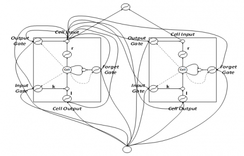
The LSTM is an RNN consisting of one or more blocks. In each LSTM block, there is a memory cell to record the cell state, an input gate to update the cell state, a forget gate to eliminate the redundant information of the cell state, and an output gate to export the final cell state. The three gates control the data inside and outside the block through multiplications and additions.
Figure 1. Structure of a single-block LSTM
The structure of a single-block LSTM is illustrated in Figure 1, where the activation function of k is sigmoid function and that of l and r is either sigmoid function or tanh function. As shown in Figure 1, the LSTM acquires activation values from the inside or outside of the memory cell via the three gates, and controls the cell state by the multiplication unit (the small circle). The input gate adds information to the cell state; the forget gate decides which information should be discarded in the block, and resets the cell state based on the activation values at l and r; the output gate regulates the output of cell state.
The unique, complex structure blesses the LSTM with the excellence in sequential tasks. Currently, two variants of the LSTM are widely adopted in time series prediction, namely, Peephole-LSTM and Coupled-LSTM. The two variants are compared with the classic LSTM as follows:
LSTM:
$\text { Input gate } \quad i_{t}=\sigma\left(W_{i} \cdot\left[h_{t-1}, x_{t}\right]+b_{i}\right)$ (1)
$\text { Cell state update } \quad \tilde{C}_{t}=\tan h\left(W_{c}\left[h_{t-1}, x_{t}\right]+b_{c}\right)$ (2)
$\text { Forget gate } \quad f_{t}=\sigma\left(W_{f} \cdot\left[h_{t-1}, x_{t}\right]+b_{f}\right)$ (3)
$\text { Cell state } \quad C_{t}=i_{t} * \tilde{C}_{t}+f_{t} * C_{t-1}$ (4)
$\text { Output gate } \quad o_{t}=\sigma\left(W_{o} \cdot\left[h_{t-1}, x_{t}\right]+b_{o}\right)$ (5)
$\text { Cell output } \quad h_{t}=o_{t} * \tanh \left(C_{t}\right)$ (6)
Peephole-LSTM:
$\text { Input gate } \quad i_{t}=\sigma\left(W_{i} \cdot\left[C_{t-1}, h_{t-1}, x_{t}\right]+b_{i}\right)$ (7)
$\text { Cell state update } \quad \tilde{C}_{t}=\tan h\left(W_{c}\left[h_{t-1}, x_{t}\right]+b_{c}\right)$ (8)
$\text { Forget gate } \quad f_{t}=\sigma\left(W_{f} \cdot\left[C_{t-1}, h_{t-1}, x_{t}\right]+b_{f}\right)$ (9)
$\text { Cell state } \quad C_{t}=i_{t} * \tilde{C}_{t}+f_{t} * C_{t-1}$ (10)
$\text { Output gate } \quad o_{t}=\sigma\left(W_{o} \cdot\left[C_{t}, h_{t-1}, x_{t}\right]+b_{o}\right)$ (11)
$\text { Cell output } \quad h_{t}=o_{t} * \tanh \left(C_{t}\right)$ (12)
Coupled-LSTM:
$\text { Forget gate } \quad f_{t}=\sigma\left(W_{f} \cdot\left[h_{t-1}, x_{t}\right]+b_{f}\right)$ (13)
$\text { Cell state update } \tilde{C}_{t}=\tan h\left(W_{C}\left[h_{t-1}, x_{t}\right]+b_{C}\right)$ (14)
$\text { Cell state } \quad C_{t}=\left(1-f_{t}\right) * \tilde{C}_{t}+f_{t} * C_{t-1}$ (15)
$\text { Output gate } \quad o_{t}=\sigma\left(W_{o} \cdot\left[h_{t-1}, x_{t}\right]+b_{o}\right)$ (16)
$\text { Cell output } \quad h_{t}=o_{t} * \tanh \left(C_{t}\right)$ (17)
where, $x_{t}$ is the input at time t; $W_{i}, W_{f}, W_{c}, \text { and } W_{o}$ are the weights of input gate, forget gate, cell, and output gate, respectively; $b_{i}, b_{f}, b_{c}, \text { and } b_{o}$ are the biases of input gate, forget gate, cell, and output gate, respectively; $i_{t}, f_{t} \text { and } o_{t}$ are the activation values of input gate, forget gate and output gate, respectively, $h_{t}$ is the output value at time t.
2.2 Nadam algorithm
In the field of DL, the choice of optimization algorithm is critical to model training. This paper selects the Nadam algorithm [12], a DL optimization algorithm with adaptive learning rate, to optimize our model.
Nadam algorithm inherits all the merits of another adaptive learning optimization algorithm: Adam optimization algorithm (AOA), and outperforms the AOA in the control of learning rate. Besides, the Nadam algorithm can effectively regulate gradient update. It can converge rapidly to the global optimal solution without consuming lots of memory.
The DL models trained by Nadam generally converge faster than those trained by other optimization algorithms. Therefore, Nadam algorithm has been widely applied in DL tasks with large datasets and high-dimensional spaces.
Based on the techniques introduced above, this section explains how to construct the MC-LSTM model and optimize the model through training.
3.1 Model construction
According to the introduction in subsection 2.1, the structure of the LSTM block directly bears on the forecast effect. Many scholars have explored the block structure, especially the gate arrangement.
(1) Greff et al. compared the learning effects of popular LSTM variants on different datasets, and drew two important conclusions: forget gate and output gate have greater impacts on the learning effect than input gate; Coupled-LSTM has comparable, if not better, learning effect as the classic LSTM in individual tasks.
(2) Zhou et al. [13] modified the gated recurrent unit (GRU) model into a simple LSTM with forget gate only, and proved the good overall performance of the simple model.
(3) Jozefowicz et al. [14] conducted contrastive experiments on 10,000 RNNs. The experimental results reveal that forget gate and input gate are much more important than the output gate, and that the LSTM and its variants have similar learning effects.
The above research shows the importance of the various gates to the LSTM, especially the forget gate. The learning effect of the LSTM is ultimately affected by the forget gate. Removing the other gates will not suppress the learning effect, but speed up the training.
Therefore, this paper further simplifies the Coupled-LSTM into the MC-LSTM, which only contains the forget gate. The simplification reduces the number of parameters and promotes the training speed. Note that the Coupled-LSTM, as a simplified version of classic LSTM, has no input gate.
3.2 Model structure
The MC-LSTM model retains the coupling structure of the Coupled LSTM, while removing the output gate. The two major functions of the output gate, namely, switch control and cell state activation, are transferred to the forget gate. Then, the MC-LSTM model can be expressed as:
MC-LSTM:
$\text { Forget gate } \quad f_{t}=\sigma\left(W_{f} \cdot\left[h_{t-1}, x_{t}\right]+b_{f}\right)$ (18)
$\text { Cell state update } \tilde{C}_{t}=\tan h\left(W_{C}\left[h_{t-1}, x_{t}\right]+b_{C}\right)$ (19)
$\text { Cell state } \quad C_{t}=\left(1-f_{t}\right) * \tilde{C}_{t}+f_{t} * C_{t-1}$ (20)
$\text { Cell output } \quad h_{t}=f_{t} * \tanh \left(C_{t}\right)$ (21)
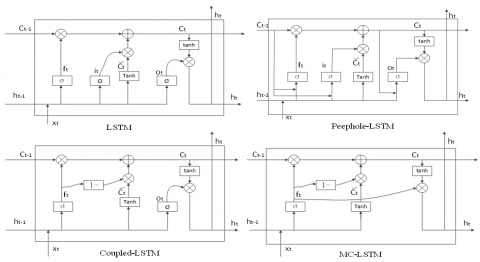
The structures of the LSTM, Peephole-LSTM, Coupled-LSTM and MC-LSTM are compared in Figure 2 below.
Figure 2. Structures of LSTM, Peephole-LSTM, Coupled-LSTM and MC-LSTM
3.3 Model optimization
The prediction effect of the MC-LSTM depends on the convergence. To improve the convergence, this paper adopts Nadam algorithm to optimize the MC-LSTM model through training.
Four parameters of Nadam algorithm must be controlled to ensure the training quality: the learning rate (α), the exponential decay rate of the first-order moment estimation (β1), the exponential decay rate of the second moment estimation (β2), and the hyper-parameter (ε) to prevent the denominator from being zero.
During model training, the four parameters were configured according to the general settings of the DL platform TensorFlow: α=0.001, β1=0.9, β2=0.999 and ε=1e-08. Under these settings, the MC-LSTM was optimized by Nadam algorithm through the following process:
|
|
Inputs: The total number of layers L; the number of neurons in each hidden layer and the output layer; the activation function; the loss function; the iterative step h; the maximum number of iterations MAX; the termination threshold j; the number of training samples m. |
|
|
Outputs: The weights W and biases b of each hidden layer and the output layer. |
|
1 |
Randomly initialize weights W and biases b of each hidden layer and the output layer. |
|
2 |
for iter from 1 to MAX: |
|
3 |
for i=1 to m: calculate activation value through forward propagation. |
|
4 |
for l=2 to L: calculate activation value through forward propagation. |
|
5 |
Calculate the gradient of the output layer by mean squared loss function. |
|
6 |
for l=L to 2, calculate the gradient of each layer through backpropagation. |
|
7 |
for l=2 to L, update the weights W and biases b of the first layer by Nadam algorithm. |
|
8 |
If the variations in weights W and biases b are below the termination threshold j, go to Step 9. |
|
9 |
Output weights W and biases b of each hidden layer and the output layer. |
4.1 Experimental environment
This section attempts to verify the effectiveness of the MC-LSTM through contrastive experiments. The experiments were carried out on a computer operating on Ubuntu 16.04 (64bit) with an Intel Core i7-8700 CPU (memory: 16GB) and a GeForce GTX1060 GPU. The software system consists of the TensorFlow DL framework embedded in the integrated development environment of PyCharm Community Edition (64bit). Many Python libraries are installed in the development environment, including sklearn, panda and numpy.
4.2 Feature selection
The features that greatly affect the learning effect of the MC-LSTM must be selected and constructed reasonably. Through detailed analysis on original OCH data, this paper identifies the following key features: period, temperature, air quality, area ID, congestion, and supply-demand gap. Note that the original OCH data were provided by DiDi.
The period feature was constructed based on time attributes and the events in each period. It is easier to take a ride outside the peak hours, holidays and the duration of major events. For temperature and air quality, the OCH demand plunges in unfavorable weather, such as high temperature and haze. The area ID and congestion reflect the regional difference in OCH demand across the target city. The supply-demand gap at the current moment depends on that at the previous moment. Hence, the supply-demand gap in the past can greatly affect the forecast of future gap values.
4.3 Data processing and evaluation indices
The original OCH data were collected in the following manner: First, the target city was divided into 58 areas of equal size, and each day was split into 144 10min slices; then, the data on each area were obtained every other 10min from 0:00 to 24:00 on each day. In this way, a total of 200,448 pieces of data was obtained for our experiments.
Table 1. Feature dataset
|
Time |
Region_ID |
Temp |
PM 2.5 |
Traffic |
Date |
L-GAP |
|
5:20:00-5:30:00 |
3 |
6 |
75 |
1067 |
1 |
0 |
|
5:30:00-5:40:00 |
3 |
6 |
75 |
1073 |
1 |
0 |
|
5:40:00-5:50:00 |
3 |
6 |
72 |
1097 |
1 |
1 |
|
5:50:00-6:00:00 |
3 |
6 |
72 |
901 |
1 |
0 |
|
6:00:00-6:10:00 |
3 |
6 |
72 |
1043 |
1 |
0 |
|
6:10:00-6:20:00 |
3 |
6 |
72 |
1317 |
1 |
2 |
|
6:20:00-6:30:00 |
3 |
6 |
72 |
1309 |
1 |
1 |
|
6:30:00-6:40:00 |
3 |
6 |
72 |
1393 |
1 |
0 |
|
6:40:00-6:50:00 |
3 |
6 |
72 |
1476 |
1 |
0 |
|
6:50:00-7:00:00 |
3 |
6 |
64 |
1576 |
1 |
3 |
|
7:00:00-7:10:00 |
3 |
6 |
64 |
1638 |
5 |
1 |
|
7:10:00-7:20:00 |
3 |
6 |
64 |
1991 |
5 |
2 |
|
7:20:00-7:30:00 |
3 |
6 |
64 |
1983 |
5 |
4 |
|
7:30:00-7:40:00 |
3 |
6 |
64 |
1990 |
5 |
8 |
|
7:40:00-7:50:00 |
3 |
6 |
64 |
2237 |
5 |
14 |
|
7:50:00-8:00:00 |
3 |
6 |
64 |
2239 |
5 |
21 |
|
8:00:00-8:10:00 |
3 |
6 |
64 |
2454 |
5 |
41 |
|
8:10:00-8:20:00 |
3 |
6 |
64 |
2430 |
5 |
37 |
|
8:20:00-8:30:00 |
3 |
6 |
64 |
2411 |
5 |
30 |
The original OCH data contain lots of missing entries, redundant information and entries in wrong format. These defects must be eliminated before OCH supply-demand forecast. Since the forecast is a task of time-series prediction, the processed data should be sorted in time order, creating a time series.
Here, the original data are sorted out at an interval of 10min. Then, the data were subjected to outlier elimination, normalization, conversion, query and standardization. Firstly, the original data files were converted into the CSV format and stored in a special MongoDB database. Next, the CSV files were viewed, managed and queried through the graphic interface of the database, and then stored in CSV format again.
The processed data have few outliers and high integrity, and are in the input and output formats required by the MC-LSTM model. Then, the data were divided into a training set (80%) and a test set (20%).
The final feature dataset is provided in Table 1 above, where Time is the data collection interval (10min), Region_ID is the area ID, Temp is the temperature, PM2.5 is the air quality, Traffic is the congestion, Date is the period, and L-GAP is the supply-demand gap.
The OCH supply-demand forecast effects of the MC-LSTM and contrastive models are evaluated by three indices: mean absolute error (MAE) and root-mean-square error (RMSE):
$M A E=\frac{1}{\mathrm{m}} \sum_{i=1}^{m}\left|\left(y_{i}-\hat{y}_{i}\right)\right|$ (22)
$R M S E=\sqrt{\frac{1}{m} \sum_{i=1}^{m}\left(y_{i}-\hat{y}_{i}\right)^{2}}$ (23)
where, yi and $\widehat{y}$i are predicted value and actual value, respectively. The forecast quality is negatively correlated with the MAE and RMSE values.
4.4 Results analysis
In this subsection, the OCH supply-demand forecast effect of the proposed single-gate MC-LSTM model is compared with that of several commonly used models on the experimental dataset, and the optimization effect of the Nadam algorithm was compared with that of other optimization algorithms.
4.4.1 Training speed
Figure 3. Training speeds of four models
Figure 3 compares the LSTM, Peephole-LSTM, Coupled-LSTM and MC-LSTM in terms of the average time consumed in each iteration. The four models were trained separately with the above-mentioned GPU and the CPU. The results show that the MC-LSTM consumed fewer time on average than the other models in each iteration in both GPU and CPU trainings. Besides, the GPU trainings consumed a shorter average time in each iteration than the CPU trainings. This means the single-gate MC-LSTM boasts the fastest training among the four models.
4.4.2 Prediction effect
Table 2 compares the OCH supply-demand forecast results of the MC-LSTM model on the experimental dataset with those of five models, namely, Peephole-LSTM, Coupled-LSTM, LSTM, gradient boosting decision tree (GBDT), and support vector regression (SVR). To eliminate stochasticity, 30 comparative experiments were carried out, and the mean values of these experiments were taken as the final results.
Table 2. Prediction results of different models
|
Evaluation indices
Models |
MAE |
RMSE |
|
MC-LSTM |
6.532 |
16.562 |
|
Coupled-LSTM |
7.026 |
18.211 |
|
Peephole-LSTM |
8.435 |
17.692 |
|
LSTM |
8.731 |
20.234 |
|
GBDT |
10.176 |
40.734 |
|
SVR |
13.205 |
45.157 |
As shown in Table 2, the MC-LSTM model achieved a smaller MAE and RMSE than the contrastive models, indicating that our model have excellent forecast effect on OCH supply-demand. Moreover, the deep learning models (MC-LSTM, Coupled-LSTM, Peephole-LSTM and LSTM) outperformed the GBDT and SVR in both MAE and RMSE. Overall, the single-gate MC-LSTM has the best forecast effect on OCH supply-demand.
4.4.3 Optimization effect
The proposed MC-LSTM models were separately trained by Nadam algorithm, the AOA, the stochastic gradient descent (SGD) algorithm, and the NAG algorithm, and then applied to forecast the OCH supply-demand. To eliminate stochasticity, 30 comparative experiments were carried out, and the mean values of these experiments were taken as the final results. Table 3 compares the MAEs and RMSEs of the four trained MC-LSTMs.
Table 3. Prediction results of MC-LSTMs trained by different optimization algorithms
|
Evaluation indices
Optimization algorithms |
MAE |
RMSE |
|
SGD |
8.532 |
18.562 |
|
NAG |
8.731 |
16.734 |
|
AOA |
6.532 |
16.562 |
|
Nadam |
5.026 |
14.211 |
As shown in Table 3, the MC-LSTM trained by Nadam algorithm had the lowest MAE and RMSE among the four contrastive models. This means Nadam algorithm can effectively improve the prediction effect of the MC-LSTM.
This paper mainly proposes a DL-based OCH supply-demand forecast model. Firstly, the LSTM and its variants were introduced, and the Coupled-LSTM was selected as the basis of modelling. Then, the single-gate MC-LSTM model was established and optimized by Nadam algorithm. After that, the original OCH data provided by DiDi were processed, and then divided into a training set and a test set. The superiority of the MC-LSTM model in OCH supply-demand forecast was confirmed through contrastive experiments. The research findings provide a desirable tool for OCH enterprises to forecast the supply-demand gap, reduce waiting time and make full use of vehicle resources.
In the future research, model structures other than LSTM and its variants will be introduced to OCH supply-demand forecast, and various DL techniques will be employed to enhance the prediction effect.
The work was supported by the Natural Science Foundation of Inner Mongolia (Grant No.: 2013MS0920), and Science and Technology Planning Project of Inner Mongolia (Grant No.: 201502015).
[1] Daws, M. (2016). Perspectives on the ride sourcing revolution: Surveying individual attitudes toward Uber and Lyft to inform urban transportation policymaking. Massachusetts Institute of Technology, 2016.
[2] Saadi, I., Wong, M., Farooq, B., Teller, J., Cools, M. (2017). An investigation into machine learning approaches for forecasting Spatio-temporal demand in ride-hailing service. Computer Science, 1703.02433.
[3] Wang, D., Cao, W., Li, J., Ye, J.P. (2017). DeepSD: supply-demand prediction for online car-hailing services using deep neural networks. 2017 IEEE 33rd International Conference on Data Engineering (ICDE), San Diego, CA, USA, pp. 243-254. https://doi.org/10.1109/ICDE.2017.83
[4] Li, J., Wang, Z. (2017). Online car-hailing dispatch: Deep supply-demand gap forecast on spark. IEEE 2nd International Conference on Big Data Analysis (ICBDA). IEEE, Beijing, China, 2017, pp. 811-815. https://doi.org/10.1109/ICBDA.2017.8078750
[5] Jordan, M.I., Mitchell, T.M. (2015). Machine learning: Trends, perspectives, and prospects. Science, 349(6245): 255-260. https://doi.org/10.1126/science.aaa8415
[6] Lecun, Y., Bengio, Y., Hinton, G. (2015). Deep learning. Nature, 521(7553): 436.
[7] Daniel, G. (2013). Principles of artificial neural networks. World Scientific. ISBN-13: 978-9814522731.
[8] Graves, A. (2012). Supervised Sequence Labelling with Recurrent Neural Networks. Studies in Computational Intelligence, 385. ISBN-13: 978-3642247965.
[9] Gers, F. (2001). Long short-term memory in recurrent neural networks. Learn Neural Networks.
[10] Gers, F.A., Schmidhuber, J. (2000). Recurrent nets that time and count., Proceedings of the IEEE-INNS-ENNS International Joint Conference on Neural Networks. IJCNN 2000. Neural Computing: New Challenges and Perspectives for the New Millennium, IEEE, 3: 189-194. https://doi.org/10.1109/IJCNN.2000.861302
[11] Greff, K., Srivastava, R.K., Koutnik, J., Steunebrink, B.R., Schmidhuber, J. (2017). LSTM: A search space odyssey. IEEE Transactions on Neural Networks and Learning Systems, 28(10): 2222-2232. https://doi.org/10.1109/TNNLS.2016.2582924
[12] Dozat, T. (2016). Incorporating nesterov momentum into adam. In ICLR Workshop.
[13] Zhou, G.B., Wu, J., Zhang, C.L., Zhou, Z.H. (2016). Minimal gated unit for recurrent neural networks. International Journal of Automation and Computing, 13(3): 226-234. https://doi.org/10.1007/s11633-016-1006-2
[14] Jozefowicz R, Zaremba W, Sutskever I. (2015). An empirical exploration of recurrent network architectures. International Conference on Machine Learning, 37: 2342-2350.