Mengxia Li | Ruiquan Liao | Yong Dong*
OPEN ACCESS
This paper attempts to determine the time delay between the sequence of system behaviors and that of influencing factors on system behaviors. Firstly, a new concept was coined called the representative subsequence (RS), and the RSs of influencing factors were selected. Next, a new geometric similarity grey relational grade (GRG) model was set up to compute the time delay of each influencing factor RS relative to the sequence of system behaviors. On this basis, the time-delay corresponding to the maximum GRG was taken as the desired time-delay. The verification on actual data shows that the concept and extraction rule of the RS are feasible, and our geometric similarity GRG model outperforms the conventional model in predicting time delay. The research findings lay the basis for grey prediction modelling of time sequences and optimizing the prediction effect of grey prediction models.
grey system theory (GST), time delay, representative subsequence (RS), automatic extraction
The grey system theory (GST), pioneered Deng [1] in 1982, mainly targets a special type of uncertain systems, in which the information is partly known and partly unknown. In other words, the system has a small sample with poor information. The GST aims to extract useful data from the known information, and then describe and even control the change law of system behavior. These goals are difficult to realize by probability statistic method and fuzzy sets method. GSA has been widely used [2-9]. There are many forms of extension [10-18].
In many systems, it takes time for influencing factors to take effect. For instance, it may take years for an investment policy to stimulate economic growth, or for a population policy to affect birthrate. Therefore, these systems are referred to as having the delay feature. It is very hard to predict the change law of such a time-delay system. If the sample size is large enough (generally above 30) [19], the change law could be modelled by the statistical approach; if the sample size is small, the best solution lies in the grey prediction model with time delay.
Zhai et al. [20] is the first to introduce the time delay factor into GM (1, 1), the basic model for grey prediction, creating a new model GM (1, 2) that can better reflect the dynamic relationship between two variables. However, the time delay was determined with randomly chosen subsequences. Deng [21] combines the time delay factor and GM (1, 1) into a new model GM (1, 1| τ, γ), and takes the time delay corresponding to the maximum grey relational grade (GRG) between two sequences as the time delay of the system. This strategy is called the traversing method, as it traverses through all possible time delays. Liu [22-23] explore the stability of time-delay systems, failing to explain how to determine time delay. Zhang et al. [24] identifies the time delay accurately with the neural network (NN), but the parameters must be trained with enough samples. Li and Xie [25] sets up a model with the time delay factor to achieve high prediction accuracy. Huang [26] extends GM (1, 1| τ, γ) into GM (1, N| τ, γ), without giving the GRG model, and determines the time delay through particle swarm optimization (PSO). This approach is like the traversing method. Zhang et al. [27] proposes a multi-variable grey model with time delay, and uses the traversing method to determine the time delay. Neither is the GRG model given in this reference. Chen and Dang [28] establishes the GM (1, 1, τ) model with time delay, and modifies the adaptability of GM (1, 1). In this reference, the quantitative relationship is extracted from the grey prediction model, and the time delay is measured by the traversing method. Nonetheless, these methods cannot work in the case of multiple variables. In fact, none of the above references discuss how to determine the length and location of the data involved in the CRG calculation, which are defined as a subsequence.
Fu and Zheng [29] modifies the GM (1, N) through grey relational analysis (GRA) with time delay, and obtains the time delay of the system through four steps: specifying the length of subsequence, taking out all possible subsequences with varied start points, determining the time delay of each subsequence by the traversing method, and taking the arithmetic mean of all the time delays. On the upside, the four-step approach does not need to consider the subsequence location; on the downside, the way to identify the length of subsequence is not clearly explained. Feng [30] suggests that subsequences with different lengths may cause great difference to GM (1, 1), provided that the prediction is of the required accuracy. However, this reference does not specify how to select the suitable subsequence. Therefore, it is very meaningful to explore the way to determine the length and location of subsequences.
It worth noting that, the concept of time delay in time delayed grey model and time-delayed polynomial grey system model used [31-33], is different from that used in this paper.
Considering the above, this paper defines a new concept called the representative subsequence (RS), designs an adaptive extraction algorithm for the RS, which can determine the length and location of subsequences in an adaptive manner. Next, a geometric similarity GRG model was constructed, and coupled with the RS to identify the time delay through trial-and-error. The verification on actual data shows that our method is reasonable and effective. The research results shed new light on constructing grey prediction models.
The remainder of this paper is organized as follows: Section 2 defines the RS, sets up the adaptive extraction algorithm, and builds the geometric similarity GRG model; Section 3 determines the time delay in grey prediction model with time delay; Section 4 compares our GRG model with Deng’s model through prediction on actual data; Section 5 puts forward the conclusions.
2.1 Definition 1
Let $x_{1}^{(0)}=\left(x_{1}^{(0)}(1), x_{1}^{(0)}(2), \ldots, x_{1}^{(0)}(m)\right)$ be the sequence of system behaviors and $x_{j}^{(0)}=\left(x_{j}^{(0)}(1), x_{j}^{(0)}(2), \ldots, x_{j}^{(0)}(m)\right)(j=2, \cdots, N)$ be the sequence of influencing factors on the system behaviors. Note that $x_{1}^{(0)}(k)$ and $x_{j}^{(0)}(k)$ are from the same time point; $x_{j}^{(0)}$, (j=2,⋯,N) are system inputs and $x_{1}^{(0)}$ are system outputs.
2.2 Definition 2
Let $x_{1}^{(0)}(t)+a z_{1}^{(1)}(\mathrm{t})$= $\sum_{i=2}^{N} b_{i} x_{i}^{(1)}(t-\tau)$ be the GM (1, N, τ) model, $x_{i}^{(1)}=\left(x_{i}^{(1)}(1), x_{i}^{(1)}(2), \ldots, x_{i}^{(1)}(m)\right)$ be the first-order cumulative sequence generated from $\mathcal{X}_{i}^{(0)}$, i.e. $x_{i}^{(1)}(k)=\sum_{t=1}^{k} x_{i}^{(0)}(t)$, and $z_{1}^{(1)}(t)$ be the neighboring mean sequence generated from $x_{1}^{(1)}(t),$ i.e. $z_{1}^{(1)}(t)=\frac{1}{2}\left(x_{1}^{(1)}(t)+x_{1}^{(1)}(t-1)\right)$. Note that τ≥0 is the time delay.
Drawing on the concept of information entropy [34, 35], a sequence is more representative if its elements change more violently. The change of each element can be measured by the difference or ratio between two adjacent elements. Thus, the concept of the RS was defined as follows:
2.3 Definition 3
Let yi=(yi(1),yi(2), …,yi(m-1)), where yi(t)=x(0) 1(t+1)- x(0) 1(t), (t=1,2,⋯,m-1). For sequence x(0) i=(x(0) i(1), x(0) i(2), …,x(0) i(m)), if yi is a constant sequence, then x(0) iis a linear sequence and can be described by a linear function prediction model; otherwise, the elements falling between min{k1,k2} and max{k1,k2}+1 form a RS denoted as xid. Note k1 and k2 are the maximum and minimum number of elements, respectively.
2.4 Definition 4
The geometric similarity GRG can be defined as:
$\rho (x_{i}^{(0)},x_{j}^{(0)})=\frac{1}{m}\sum\limits_{k=1}^{m}{\frac{1}{1+\frac{1}{2}{{\varphi }_{1}}(k)+\frac{1}{2}{{\varphi }_{2}}(k)}}$ (1)
where,
$\varphi_{1}(k)=\left|\frac{\Delta_{i}(k)}{\Delta_{i 0}(k)}-\frac{\Delta_{j}(k)}{\Delta_{j 0}(k)}\right|$;
${{\varphi }_{2}}(k)=\left\{ \begin{matrix} \left| 1-\frac{{}^{{{\Delta }_{i}}(k)}/{}_{{{\Delta }_{i0}}(k)}}{{}^{{{\Delta }_{j}}(k)}/{}_{{{\Delta }_{j0}}(k)}} \right| & {{\Delta }_{j}}(k)\ne 0 \\ 1 & {{\Delta }_{j}}(k)=0 \\\end{matrix} \right.$;
$\Delta_{i}(k)=x_{i}^{(0)}(k)-x_{i}^{(0)}(1)$;
$\Delta_{i 0}(k)=\min \left\{\left(x_{i}^{(0)}(k)-x_{i}^{(0)}(1)\right) \neq 0, k=1,2, \ldots, m\right\}$;
Dj(k) and Dj0(k) have similar meanings.
The above is a GRG model satisfying the linear correlation similarity and linear correlation approximation [36].
Under the effects of the influencing factors, the system behavior system will change correspondingly, but with time delays. In this section, the time delay of each influencing factor sequence relative to the system behavior system is evaluated through the following steps.
Step 1. Let m be the maximum length of the sequence of influencing factors $x_{j}^{(0)},(j=2, \cdots, N)$. By definition, the RS xid consists of elements from $x_{i}^{(0)}$ falling between k3 and k4 with k3<k4. The length of the RS xid can be denoted as Lid.
Step 2. From the sequence of system behavior $x_{1}^{(0)}$, the elements from k3 to k4 should be selected successively at τ=0, those from k3+1 to k4+1 at τ=1, … and those from m-Lid+1 to m at τ=m-k4. The elements selected each time form a system behavior subsequence. The GRG between each system behavior subsequence and the influencing factor RS should be computed. Then, the τ corresponding to the maximum GRG is the time delay (τj, j=2,⋯,N) between $x_{j}^{(0)}$ and $\mathcal{X}_{1}^{(0)}$.
Step 3. The above steps should be repeated until the time delay between each system behavior subsequence and the influencing factor RS have been obtained.
Considering the time delay in the influence of technological progress on economic development, Fu and Zheng [12] explored the relationship between these two factors in China, and determined the time delay as two years through time-delayed grey relational analysis based on the relevant data in 2007~2015. However, the time delay thus obtained is an arithmetic mean, rather than the accurate value. As shown in Table 1, the research data, including the research and development (R&D) expenditure and gross domestic product (GDP) in that period, were collected from China Statistical Yearbooks 2011 and 2016.
Our algorithm processes these data in the following steps:
Step 1. Let $x_{j}^{(0)}$ be the extracted data on R&D expenditure, whose length is m=9. Then, we have yj=[905.8,1186.1,1260.5,1624.4,1611.4,1548.2,1169, 1154.3].
It is easy to obtain that k3=1 and k4=5. Thus, the RS can be established as $x_{i d}=\left(x_{j}^{(0)}(1), x_{j}^{(0)}(2), x_{j}^{(0)}(3), x_{j}^{(0)}(4), x_{j}^{(0)}(5)\right)$.
Step 2. The time delays and GRGs are shown in Table 2 below.
Table 1. The data used by Fu and Zheng [12] (data source: China Statistical Yearbooks)
|
Year |
GDP |
R&D expenditure |
|
2007 |
270,232.3 |
3,710.2 |
|
2008 |
319,515.5 |
4,616.0 |
|
2009 |
349,081.4 |
5,802.1 |
|
2010 |
413,030.3 |
7,062.6 |
|
2011 |
489,300.6 |
8,687.0 |
|
2012 |
540,367.4 |
10,298.4 |
|
2013 |
595,244.4 |
11,846.6 |
|
2014 |
643,974.0 |
13,015.6 |
|
2015 |
685,505.8 |
14,169.9 |
Table 2. Time delays and GRGs
|
Time delays |
t=0 |
t=1 |
t=2 |
t=3 |
t=4 |
|
GRG of our model |
0.810 |
0.647 |
0.813 |
0.765 |
0.809 |
|
GRG of Deng’s model |
0.709 |
0.674 |
0.725 |
0.683 |
0.625 |
Obviously, the time delay corresponding to the maximum grey relations is t=2. The result is the same with Fu and Zheng [12], but our result has clearer meanings than theirs.
The another actual data for verification were extracted from [37], See Table 3, which deals with one sequence of system behaviors $\mathcal{x}_{1}^{(0)}$ (China’s gross marine product, unit: RMB 100 million yuan) and two sequences of influencing factors $x_{2}^{(0)}$ (ocean industry employment, unit: 10,000 people) and $x_{3}^{(0)}$ (ocean industry fixed-asset investment, unit: RMB 100 million yuan). In this reference, the time delay between $x_{1}^{(0)}$ and $x_{2}^{(0)}$, and that between $x_{1}^{(0)}$ and $x_{3}^{(0)}$are both investigated. However, the authors of this reference did not specify how to determine the length or location of subsequences, but simply assumed that both time delays are one. Lu et al. [37] concludes that about half of the employees in the ocean industry work in fishery and related fields. Thus, increasing ocean industry employment can bolster fishing revenue and stimulate marine economy. It was also concluded that the fixed-asset investment in ocean industry has a limited impact on marine economy in China, i.e. the investment needs a long time to take effect. Hence, the time delay of $x_{1}^{(0)}$ with respect to $x_{2}^{(0)}$ is much shorter than that of $x_{1}^{(0)}$ with respect to $x_{2}^{(0)}$. Deng’s grey relational model is adopted in that reference to compute the geometrical similarity between sequences.
Table 3. Actual data: x(0) 1, x(0) 2, x(0) 3
|
Years |
2001 |
2002 |
2003 |
2004 |
2005 |
2006 |
|
$x_{1}^{(0)}$ |
9518 |
1,1403 |
11,882 |
13,890 |
16,154 |
19,062 |
|
$x_{2}^{(0)}$ |
3,135 |
3,265 |
3,057 |
3,336 |
3,432 |
3,570 |
|
$x_{3}^{(0)}$ |
2,108 |
2,277 |
2,440 |
2,536 |
2,781 |
2,960 |
|
Years |
2007 |
2008 |
2009 |
2010 |
2011 |
|
|
$x_{1}^{(0)}$ |
21,883 |
24,049 |
26,262 |
30,122 |
33,255 |
|
|
$x_{2}^{(0)}$ |
3,659 |
4,001 |
3,862 |
4,028 |
4,325 |
|
|
$x_{3}^{(0)}$ |
3,151 |
3,218 |
3,271 |
3,350 |
3,420 |
|
In this paper, our grey relational model is compared with Deng’s model through the following steps.
Step 1. Take $x_{2}^{(0)}$ as $x_{j}^{(0)}$, then m=11 and yj=[169, 163, 96, 245, 179, 191, 67, 53, 79, 70]. It is easy to obtain that k3=4 and k4=9. Thus, the RSs are $x_{i d}=\left(x_{j}^{(0)}(4), x_{j}^{(0)}(5), \ldots, x_{j}^{(0)}(9)\right)$.
Step 2. Compare the time delays and GRGs between $x_{1}^{(0)}$ and $x_{2}^{(0)}$ of the two models (Table 4).
Table 4. Time delays and GRGs between $x_{1}^{(0)}$ and $x_{2}^{(0)}$
|
Time delay |
τ=0 |
τ=1 |
τ=2 |
|
GRG of our model |
0.556 |
0.606 |
0.602 |
|
GRG of Deng’s model |
0.602 |
0.625 |
0.699 |
Obviously, the maximum GRG appears at the time delay of τ=1.
Step 3. Take $x_{3}^{(0)}$ as $x_{j}^{(0)}$ and repeat the above steps. It is easy to obtain that k3=2 and k4=8. In this case, the time delays and GRGs between $x_{1}^{(0)}$ and $x_{3}^{(0)}$ of the two models are listed in Table 5.
Table 5. Time delays and GRGs between $x_{1}^{(0)}$ and $x_{3}^{(0)}$
|
Time delay |
τ=0 |
τ=1 |
τ=2 |
τ=3 |
|
GRG of our model |
0.285 |
0.378 |
0.379 |
0.397 |
|
GRG of Deng’s model |
0.616 |
0.547 |
0.560 |
0.578 |
The time delays obtained by our model agree with the previous conclusion that the time delay of $x_{1}^{(0)}$ with respect to $x_{2}^{(0)}$ is much shorter than that of $x_{1}^{(0)}$ with respect to $x_{2}^{(0)}$.
The prediction effects of the two models are compared as follows:
The time delay determined by Fu and Zheng [37] was $\tau=[1,1]$. The discrete GM (1, N, τ) can be expressed as:
$-az_{1}^{(1)}(t)+{{b}_{2}}x_{2}^{(1)}(t-1)+{{b}_{3}}x_{3}^{(1)}(t-1)=x_{1}^{(0)}(t)$ (2)
where, t=2, 3, ⋯, 11.
Then, the following matrix equation need to be solved:
$A\left( \begin{matrix} a \\ {{b}_{2}} \\ {{b}_{3}} \\\end{matrix} \right)=C$ (3)
where,
$A=\left(\begin{array}{ccc}{-z_{1}^{(1)}(2)} & {x_{2}^{(1)}(2-1)} & {x_{3}^{(1)}(2-1)} \\ {-z_{1}^{(1)}(3)} & {x_{2}^{(1)}(3-1)} & {x_{3}^{(1)}(3-1)} \\ {\vdots} & {\vdots} & {\vdots} \\ {-z_{1}^{(1)}(11)} & {x_{2}^{(1)}(11-1)} & {x_{3}^{(1)}(11-1)}\end{array}\right) ; C=\left(\begin{array}{c}{x_{1}^{(0)}(2)} \\ {x_{1}^{(0)}(3)} \\ {\vdots} \\ {x_{1}^{(0)}(11)}\end{array}\right)$.
To solve the above matrix equation, the objective function should be constructed based on the least squares (LS):
$\min _{x} F(x)=(A x-C)^{2}$ (4)
where,\[x=\left( \begin{matrix} a \\ {{b}_{2}} \\ {{b}_{3}} \\\end{matrix} \right)$.
In this paper, the chaos simulated annealing (CSA) algorithm is established to solve x, i.e. to find the values of a, b2 and b3. To describe the CSA algorithm, the logistic chaotic mapping was introduced:
${{t}_{n+1}}=\mu \cdot {{t}_{n}}\cdot (1-{{t}_{n}})$, $n=1,2,3, \dots$ (5)
where, μ=3.98. The sequence generated by the logistic chaotic mapping carries the chaotic features, and every number in the sequence falls in the interval [0, 1].
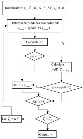
Then, the set of initial solutions was generated through logistic chaotic mapping in the following steps:
Step 1. Initialize the search space, number of dimensions, and number of initial solutions as [-M,M], N and L. Select an initial value t1=0.6935. Generate N⋅L numbers ti, i=1, 2, ⋯, N⋅L, through logistic chaotic mapping. Then, map ti to the search space and denote the result as xi:
$x_{i}=\frac{t_{i}-0.5}{0.5} M$ (6)
Create a vector based on every N numbers to serve as an initial solution. Calculate the objective function value F(xi) of each solution. Initialize the best-known solution x*, which satisfies $F\left(x^{*}\right)=\min _{i=1,2,...L} F\left(x_{i}\right)$.
Initialize the number of iterations LT corresponding to each temperature, the initial temperature T0, the lower bound of temperature Tf, the temperature attenuation coefficient 0<α<1, the current temperature Tc=T0 and the current number of iterations DC=1.
Step 2. Disturb DC=1 to generate xi-new, and compute the objective function value F(xi-new).
Step 3. Compute dE=F(xi-new)-F(xi).
Step 4. If dE<0, then let xi=xi-new and update x*. Otherwise, randomly select a p0 value, which is evenly distributed in [0, 1]; if p0<exp(-dE/Tc), xi=xi-new and update x*.
Step 5. Check the number of iterations DC. If DC=LT, go to Step 6; otherwise, go to Step 2 and let DC=DC+1.
Step 6. Check if the termination condition is satisfied. If Tc≤Tf, output x*; otherwise, let Tc=αTc and go to Step 2.
The workflow of the CSA algorithm is illustrated in Figure 1.
The time delay determined by our model was $\tau=[1,3]$. The discrete GM (1, N, τ) model can be described as:
$-a z_{1}^{(1)}(t)+b_{2} x_{2}^{(1)}(t-1)+b_{3} x_{3}^{(1)}(t-3)=x_{1}^{(0)}(t)$ (7)
where, t=4, 3, ⋯, 11.
Then, the following matrix equation should be solved:
$A_{1}\left(\begin{array}{l}{a} \\ {b_{2}} \\ {b_{3}}\end{array}\right)=C_{1}$ (8)
where,
$A_{1}=\left(\begin{array}{ccc}{-z_{1}^{(1)}(4)} & {x_{2}^{(1)}(4-1)} & {x_{3}^{(1)}(4-3)} \\ {-z_{1}^{(1)}(5)} & {x_{2}^{(1)}(5-1)} & {x_{3}^{(1)}(5-3)} \\ {\vdots} & {\vdots} & {\vdots} \\ {-z_{1}^{(1)}(11)} & {x_{2}^{(1)}(11-1)} & {x_{3}^{(1)}(11-3)}\end{array}\right), C_{1}=\left(\begin{array}{c}{x_{1}^{(0)}(4)} \\ {x_{1}^{(0)}(5)} \\ {\vdots} \\ {x_{1}^{(0)}(11)}\end{array}\right)$.
The CSA algorithm was adopted to solve the time delay model of Fu and Zheng [37] and the time delay model of our research. The parameters thus obtained are compared in Table 6.
Table 7 lists the error test results of the two models. The residual error is defined as:
$\varepsilon(k)=x_{1}^{(0)}(k)-\hat{x}_{1}^{(0)}(k)$ (9)
where, $x_{1}^{(0)}(k)$ is the actual value; $\hat{x}_{1}^{(0)}(k)$ is the simulated value.
The relative error is defined as:
$\Delta(k)=\left|\frac{\varepsilon(k)}{x_{1}^{(0)}(k)}\right|$ (10)
As shown in Table 7, our model achieved a smaller relative error than Fu and Zheng’s model. Even if only the cases 4~11 were compared, the sum of the absolute values of residual values of Fu and Zheng’s model was 6,308.45, far greater than that (2,335.04) of our model. This confirms the good simulation effect of our model.
Figure 1. Workflow of the CSA algorithm
Table 6. Coefficients of our model and Fu and Zheng’s model [37]
|
Coefficient |
-a |
b2 |
b3 |
|
Fu and Zheng’s model |
0.3313 |
10.1092 |
-13.8671 |
|
Our model |
0.0969 |
1.4760 |
-1.7937 |
Table 7. Errors of our model and Fu and Zheng’s model [37]
|
Serial number |
Actual value |
Fu and Zheng’s model [37] |
Our model |
||
|
Simulated value |
Residual error/% |
Simulated value |
Relative error/% |
||
|
1 |
9,518 |
/ |
/ |
/ |
/ |
|
2 |
11,403 |
7,501.8 |
34.2 |
/ |
/ |
|
3 |
11,882 |
12,789 |
7.64 |
/ |
/ |
|
4 |
13,890 |
14,126 |
1.70 |
14,030 |
1.01 |
|
5 |
16,154 |
17,659 |
9.32 |
16,325 |
1.06 |
|
6 |
19,062 |
19,622 |
2.94 |
18,721 |
1.79 |
|
7 |
21,883 |
21,447 |
1.99 |
21,426 |
2.09 |
|
8 |
24,049 |
22,348 |
7.07 |
24,064 |
0.06 |
|
9 |
26,262 |
26,504 |
0.92 |
27,098 |
3.18 |
|
10 |
30,122 |
29,525 |
1.98 |
29879 |
0.81 |
|
11 |
33,255 |
34,286 |
3.1 |
33,124 |
0.39 |
|
Mean |
|
|
7.09 |
|
1.30 |
In this paper, a new concept called the RS is defined, and an adaptive extraction algorithm is developed for the RS. Next, a geometric similarity GRG model was constructed, and coupled with the RS to identify the time delay through trial-and-error. The verification on actual data shows that the RS is a feasible concept; our grey relational model outperforms Deng’s model in predicting the geometrical similarity of sequences; the combination between the RS and our model can accurately identify the time delays between sequences.
The authors will thank people in the Branch of Key Laboratory of CNPC for Oil and Gas Production for their great help. This paper is supported by National Natural Science Foundation of China (61572084 and 51504038), National Key S&T Special Projects (2016ZX05056004-002 and 2016ZX05046004-003), and China Petroleum Innovation Fund Project (2015D-5006-0208). This paper is also supported by Educational Commission of Hubei Province of China (Q20171302) and University-level teaching and research project (JY2017014).
[1] Deng, J.L. (2005). Basic Method of Grey System (Edition 1). Wuhan: Huazhong University of Science and Technology Press, 2-22.
[2] Shen, V.R., Chung, Y.F., Chen, T.S. (2009). A novel application of grey system theory to information security (Part I). Computer Standards & Interfaces, 31(2): 277-281. https://doi.org/10.1016/j.csi.2007.11.018
[3] Li, G.D., Masuda, S., Nagai, M. (2013). The prediction model for electrical power system using an improved hybrid optimization model. International Journal of Electrical Power & Energy Systems, 44(1): 981-987. https://doi.org/10.1016/j.ijepes.2012.08.047
[4] Chang, E.C., Xu, Z., Su, Z., Wu, R.C. (2015). Fuzzy grey predictor compensated time-varying variable structure controller for solar inverters. Journal of Intelligent & Fuzzy Systems, 29(6): 2597-2602. https://doi.org/10.3233/IFS-151962
[5] Goshu, N.N., Tilahun, S.L. (2016). Grey theory to predict Ethiopian foreign currency exchange rate. International Journal of Business Forecasting and Marketing Intelligence, 2(2): 95-116. https://doi.org/10.1504/IJBFMI.2016.078148
[6] Becker, U., Manz, H. (2016). Grey systems theory time series prediction applied to road traffic safety in Germany. IFAC-PapersOnLine, 49(3): 231-236. https://doi.org/10.1016/j.ifacol.2016.07.039
[7] Bezuglov, A., Comert, G. (2016). Short-term freeway traffic parameter prediction: Application of grey system theory models. Expert Systems with Applications, 62: 284-292. https://doi.org/10.1016/j.eswa.2016.06.032
[8] Ding, S. (2019). A novel discrete grey multivariable model and its application in forecasting the output value of China’s high-tech industries. Computers & Industrial Engineering, 127: 749-760. https://doi.org/10.1016/j.cie.2018.11.016
[9] Qiao, X., Zhang, Z., Jiang, X., He, Y., Li, X. (2019). Application of grey theory in pollution prediction on insulator surface in power systems. Engineering Failure Analysis, 106: 104153. https://doi.org/10.1016/j.engfailanal.2019.104153
[10] Li, G.D., Yamaguchi, D., Nagai, M., Masuda, S. (2008). The prediction of asphalt pavement permanent deformation by T-GM (1, 2) dynamic model. International Journal of Systems Science, 39(10): 959-967. https://doi.org/10.1080/00207720801979927
[11] Li, Z., Ho, Y.S. (2008). Use of citation per publication as an indicator to evaluate contingent valuation research. Scientometrics, 75(1): 97-110. https://doi.org/10.1007/s11192-007-1838-1
[12] Lu, H.S., Chang, C.K., Hwanga, N.C., Chung, C.T. (2009). Grey relational analysis coupled with principal component analysis for optimization design of the cutting parameters in high speed end milling. Journal of Materials Processing Technology, 209(8): 3808-3817. https://doi.org/10.14741/Ijcet/Spl.2.2014.05
[13] Tien, T.L. (2009). A new grey prediction model FGM(1, 1). Mathematical and Computer Modelling, 49(7-8): 1416-1426. https://doi.org/10.1016/j.mcm.2008.11.015
[14] Tung, C.T., Lee, Y.J., Wang, K.H. (2009). Combining grey theory and principal component analysis to evaluate financial performance of airline companies in Taiwan. Journal of Grey System, 21(4): 357-368.
[15] Hsiao, Y.T., Huang, T.L., Chang, S.Y. (2011). Fuzzy modeling with grey prediction for designing power system stabilizers. Granular Computing and Intelligence Systems, 13: 219-235. https://doi.org/10.1007/978-3-642-19820-5_11
[16] Yin, M.S. (2013). Fifteen years of grey system theory research: A historical review and bibliometric analysis. Expert systems with Applications, 40(7): 2767-2775. https://doi.org/10.1016/j.eswa.2012.11.002
[17] Wu, L., Liu, S., Yao, L., Xu, R., Lei, X. (2015). Using fractional order accumulation to reduce errors from inverse accumulated generating operator of grey model. Soft Computing, 19(2): 483-488. https://doi.org/10.1007/s00500-014-1268-y
[18] Kumar, R.S., Ganesh, G.S., Vijayarangan, N., Padmanabhan, K., Satish, B., Kumar, A. (2017). Machine learning grey model for prediction. 2017 International Conference on Computational Science and Computational Intelligence (CSCI), Las Vegas, NV, USA. http://dx.doi.org/10.1109/CSCI.2017.138
[19] Liu, S.F., Dang, Y.G., Fang, Z.G., Xie, N.M. (2010). Grey System Theory and Its Application. Beijing: Science Press, 1-27.
[20] Zhai, J., Feng, Y.J., Sheng, J.M. (1996). A time-lag-existing GM(1,2) model and its application. Systems Engineering, (6): 51, 66-68.
[21] Deng, J.L. (2001). A novel grey model GM(1, 1|τ, r) generalizing GM(1, 1). Journal of Grey System, 13(1): 1-8.
[22] Liu, P.L. (2001). Stability of continuous and discrete time-delay grey systems. International Journal of Systems Science, 32(7): 947-952. https://doi.org/10.1080/00207720010005636
[23] Liu, P.L. (2001). Robustness of pole assignment in a specified circular region for discrete-time grey systems. International Journal of Systems Science, 32(2): 269-272. https://doi.org/10.1080/00207720120717
[24] Zhang, Z.Y., Liu, X., Huang, C.X. (2012). Fuzzy-control with gray-predictor for time-varying delay systems. Applied Mechanics and Materials, 1487(109): 306-310. http://dx.doi.org/10.4028/www.scientific.net/AMM.109.306
[25] Li, C., Xie, X.P. (2019). GM(1,1|τi) prediction model with time-varying delay function and its application. Systems Engineering - Theory & Practice, 39(6): 1535-1549.
[26] Huang, J. (2009). Grey GM(1, N|τ, r) model and its particle swarm optimization algorithm. Systems Engineering - Theory & Practice, 29(10): 145-151. https://doi.org/10.3321/j.issn:1000-6788.2009.10.018
[27] Zhang, K., Qu, P.P., Zhang, Y.T. (2015). Delay multi-variables discrete grey model and its application. Systems Engineering - Theory & Practice, 35(8): 2092-2103. http://www.sysengi.com/CN/10.12011/1000-6788(2015)8-2092
[28] Chen, X.Y., Dang, Y.G. (2015). Grey GM(1, 1, τ) model with time delay parameter and its application. Mathematics in Practice and Theory, 45(4): 95-100.
[29] Fu, Z.H., Zheng, R.J. (2018). Multivariable time-delayed GM(1,N) coordination degree model and its application. Statistics & Decision, 34(13): 77-80.
[30] Feng, L.H. (1997). Discussion of the problem of grey forecast model. Systems Engineering - Theory & Practice, (12): 126-129, 138.
[31] Ma, X., Liu, Z.B. (2017). Application of a novel time-delayed polynomial grey model to predict the natural gas consumption in China. Journal of Computational and Applied Mathematics, 324: 17-24. http://dx.doi.org/10.1016/j.cam.2017.04.020
[32] Ma, X., Mei, X., Wu, W.Q., Wu, X.X., Zeng, B. (2019). A novel fractional time delayed grey model with Grey Wolf Optimizer and its applications in forecasting the natural gas and coal consumption in Chongqing China. Energy, 178: 487-507. http://dx.doi.org/10.1016/j.energy.2019. 04.096
[33] Chen, L., Liu, Z.B., Ma, N.N. (2018). Time-delayed polynomial grey system model with the fractional order accumulation. Mathematical Problems in Engineering, (3640625): 1-7. https://doi.org/10.1155/2018/3640625
[34] Li, G.L., Fu, Q. (2006). Grey relational analysis model based on weighted entropy and its Application. 2007 International Conference on Wireless Communications, Networking and Mobile Computing, Shanghai, China. https://doi.org/10.1109/WICOM.2007.1347
[35] Chen, L.R., Guo, J.W., Wang, J.M. (2005). Application of the gray relevant analysis based on entropy in evaluating competition of power enterprises. Journal of Electric Power, 20(4): 359-361.
[36] Wei, Y., Zeng, K.F. (2015). The simplified relational axioms and the axiomatic definition of special incidence degrees. Systems Engineering - Theory & Practice, 35(6): 1528-1534.
[37] Lu, Y.Y., Yuan, F., Tan, D.Z. (2014). Time-delayed GM(1, N) model and its application. Statistics & Decision, 30(14): 73-75.