Fitri Indriastiwi* | S. P. Hadiwardoyo | Nahry
© 2023 IIETA. This article is published by IIETA and is licensed under the CC BY 4.0 license (http://creativecommons.org/licenses/by/4.0/).
OPEN ACCESS
Freight transportation has an essential role in connecting supply and demand that are spread geographically, which impacts the region’s economic. In an archipelagic country like, Indonesia, freight transportation ideally involves more than one mode or multimodal transport. Currently, the development of transportation infrastructure networks is not yet integrated and lacks a multimodal perspective. Meanwhile, many stakeholders or actors involved in the freight transport sector also increase the complexity of multimodal network planning. From the government perspective, each transportation sub-sectors, primarily based on the mode, has its planning and lacks integration, particularly in multimodal transport. This paper proposes the integrated strategic planning model of a multimodal freight transport network. It emphasizes how to attain the optimum benefit which represents the efficient value in the freight transport system. The model’s objective is to minimize the total distribution cost of the whole system by using the budget limitation of the transportation infrastructure’s total investment, operational and maintenance cost. The budget limitation constraint indeed represents the role of the government to arrange the budget for the transportation sub-sector. The results showed that this model can select the best scenario of infrastructure development from the perspective of multimodal transport rather than unimodal. The proposed model can be used to integrate the planning of the transportation sub-sectors and, at the same time, develop more optimum multimodal transportation system.
integrated planning, multimodal network, freight transport, generalized transport cost
Freight transportation has a vital role in the supply chain. Freight transportation connecting supply-based regions and demand-based regions ensures the availability of raw materials and finished products on time geographically [1].
For example, Indonesia’s freight transportation network in archipelago countries will involve more than one mode, thus using multimodal transport. Multimodal transport consists of long-haul transportation that uses sea, rail, air transportation, pre-haul and post-haul using land transportation or functions as inland transport (transportation to the hinterland) SteadieSeifi et al. [2]. Therefore, treating the freight transport network as a multimodal transport network is essential.
Multimodal transport has the potential to provide better overall efficiency, such as economic and performance aspects, as well as lower environmental and social impacts. However, the practical evaluation of such externalities would allow a more realistic estimation of the total costs of transport, thus increasing the opportunities of multimodal transport in terms of competition with all road transport [3]. Multimodal transport will be more competitive when it can reduce total logistics costs and provide competitive transit times, prices and performance.
The freight transport network model helps support policy design at the strategic planning level. As a result, multimodal freight transportation gets more attention at the strategic planning level. American and European Countries have improved multimodal freight transportation network design related to strategic planning and policies, while Asian countries have lagged [4].
Strategic planning problems relate to investment decisions on the present infrastructure networks [2]. However, the lack of freight transport from the multimodal perspective can be used as a policy tool to integrate freight transport development [5]. Many stakeholders or actors involved in the freight transport sector also increase the complexity of multimodal network planning.
Meanwhile, the strategic planning level in the multimodal perspective will give insight to the various stakeholders of freight transport. For example, the government or policymaker, operator transportation, or transport companies can get insight into policy measure analysis, capacity infrastructure, transport planning and social context related to environmental issues [6].
From the governmental perspective, a freight transport model is used for decision-making in transportation policies such as changes to national regulations, taxes, or infrastructure investment in particular links, nodes and corridors, construction of new roads, railways, canals, ports, multimodal terminals. etc.), traffic management and policies related to pricing, such as road pricing, charges on rail infrastructure, emission-free zones, etc. [7]. However, Kramarz et al. [8] found that the policymaker and other stakeholders determine transport development. Therefore, each of them has its respective purpose.
The freight transport network consists of sea, road, rail and air. Ideally, the transport network should integrate the infrastructure, regulation and institutions, including budgeting schemes and financing [9]. For some countries, for example, Indonesia, their freight transport systems still need significant development and political will as the freight transport infrastructure planning is still lacked integration. As of the government side, currently each transport sector has its own planning, including budget planning. It needs the integrated infrastructure planning, namely the integrated planning with a multimodal perspective. It does not just consider unimodal but multimodal as a whole system. Accordingly, in term of budget, the national transportation budget should be allocated to each sector also in the context of multimodal system, i.e., a total multimodal network system, not partially per sector.
This paper addresses a strategic freight transport planning model that focuses on the integration of transport sectors under multimodal perspective. This paper contributes an innovative integrated planning framework applied to the freight transport network model. The objective of the model is minimizing the total distribution cost of the system and maximizing the benefit that represent with efficiency value, while consider the budget limitations. This paper also provides the tools to support the decision-making process on the infrastructure development through some scenarios defined by the government. One of the scenarios may prioritize the development of rail mode over other modes. Globally, the development of rail mode needs intervention to support their share due to its advantage in term of sustainable. It is relevant to the notions that rail mode needs strategies to improve and can compete with the other modes [10].
The remainder of the paper is organized as follows: Section 2 presents comprehensive review of the state of the relevant literature; in Section 3 formulations of integrated multimodal freight network design model and components in details including the building of network representation is mentioned. In Section 4, the results from analysis using simple network is given, and finally, in Section 5, conclusion along with the potential future research is mentioned.
The model of transport development initially adopts a unimodal approach. Consequently, road and rail construction projects are planned and built separately without considering the future possibility of integration. The multimodal planning then becomes important to consider planning freight transport development.
Based on the time horizon, the planning issues are often characterized by strategic, tactical and operational planning. The most recent review of multimodal planning by SteadieSeifi et al. [2] showed that strategic planning problems are related to decisions about the investment in the present network infrastructures. Mostly, the research about strategic planning related to consolidation systems configured as hub-and-spoke networks. These problems are called hub location problems, with the hub being a freight handling (consolidation) facility. Locations of hubs are determined, and spoke nodes are allocated to the hubs. Meanwhile, according to reference [11], the strategic level also means that the research applied to a national scale and did not consider the logistic aspect at the company level and multiple levels such as the logistic level. Regarding the latter, it is essential to underline that an intermodal node’s function should be interpreted on several territorial scales [12]. Based on that, the analysis of this research can be described at a national or regional.
Currently, many types of research have been carried out and have produced various policies to improve the implementation of freight transport [13]. Zhang et al. [14] introduced model that accounts for the interaction between the infrastructure network, service network and regulatory policies that were considered from the governmental perspective and could be used for strategic network design in the mediumto long-term introduced. While Chang [15] showed that network planning involves multi-criteria decision-making to minimize costs, time and carbon emissions as well as increase service levels and utilization. Moreover, Yamada et al. [16] introduced a model for strategic transport planning, particularly in freight terminal development and interregional freight transport network, for minimizing the network costs from the governmental perspective and the route costs from the network users’ perspective. Further, a model that evaluates several policy scenarios by estimating the system cost of the transportation network was proposed by Sjafruddin et al. [17]. Related to the cost of multimodal freight transport, Beuthe et al. [18] simulated freight flows in a real network as an impact of internalizing external cost. Geerts et al. [19] developed extended freight transport model to analyse the impact of several scenario modifying the infrastructure network, internalizing external cost and extra operating time. Then the model improved by Limbourg and Jourquin [20] developed a hub allocation model for optimal locations with a certain number of hubs and candidate locations. Jonkeren et al. [21] also applied this model to estimate the impact of the market share of inland waterway transport in Europe as the impact of climate change. In comparison, the extension of this model addresses the importance of integrating service networks [22]. Bilegan et al. [23] studied the service network in tactical planning that considers revenue management with the various combinations of customer categories, fare classes and decision-making policies.
3.1 The planning process of freight transportation infrastructure
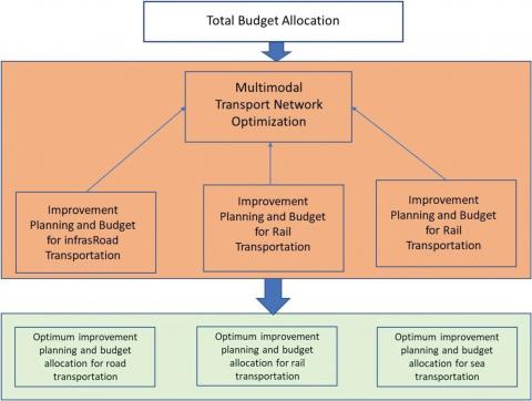
As the aim of this study, our proposed strategic planning model focuses on the integration of transport sectors under a multimodal perspective. The model’s objective is to minimize the total distribution cost of the system and maximize the efficiency value while considering the budget limitations. On the contrary, from a unimodal perspective, each transportation sector has its planning and budget allocation. Each sector or mode of transportation conducts system optimization and development of its plans, so each sector’s optimal development and budget allocation lack dependency on the other sectors. The iterations to fit the total national budget for the development of all sectors are often resulted in an inefficient planning process. Therefore, it is necessary to review the planning and optimize the network system to obtain the optimal strategy and new budget allocation. The planning process under unimodal perspective can be seen in Figure 1.
This research proposes a model that can optimize multimodal transportation networks where the development plan and budget allocation for each sector are obtained using a multimodal transportation network. Similarly, this model also considers the total national budget. However, the multimodal optimization approach may avoid inefficient iterative budget allocation. This model is expected to produce better efficiency in the planning process. The planning process can be seen in Figure 2.
Figure 1. Transportation infrastructure planning process in the unimodal perspective
Figure 2. Transportation infrastructure planning process in the multimodal perspective under budget limitation
3.2 Research framework
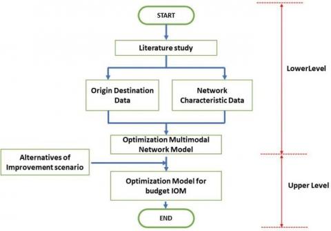
Based on the planning process, the research framework can be described as follows. The research begins with a literature study to find out the related strategic planning and optimization freight transport network. Then, identify the variables for input in the model such as network characteristic, origin and destination data. Then, build a multimodal freight transport network model to perform the optimization of the multimodal freight transport network using a genetic algorithm. Bi-level programming is using with the upper level constrained by the results of the lower level. The goal at the lower level is to minimize costs (minimize generalized transport costs), while at the upper level it is to maximize benefits, along with the various development scenarios, the framework can be seen in full in Figure 3.
In the scenario selection, the objective is optimization to get the minimum total distribution cost of system, considering the investment, operational, maintenance (IOM).
3.3 Multimodal freight network design model
This study determines the optimal combination of several development on links (such as road and rails) to reduce travel time and also on nodes (such as ports and rail terminals) to reduce transshipment costs and transfer time on multimodal connections. The combination of development using the optimistic, moderate and pessimistic scenarios.
Figure 3. Research framework
As the basis of a transportation network model, the graph model mainly consists of nodes connected by a set of links [24]. Graph G represents G(N,L), N is a set of nodes and L represents a link. Nodes in the transportation network comprise centroid nodes that represent the beginning or end of the trips. Node is also represented terminal, e.g., port, rail terminal or dry port. While the link connects nodes. Links have several network attributes such as distances, link cost (\$/km), transshipment cost (\$/ton), transshipment time (hour), the value of time (\$/ hour), the value of reliability (\$/hour) and freight flow on the respective link (ton).
Costs that consider monetary cost elements and non-monetary cost elements of a journey or externalities cost are called generalized transport costs [25]. The non-monetary cost that important to be considered and has significant impact in terms of total generalized transport cost are value of time and value of reliability. value of time is the monetary value that the decision-maker (shipper/freight forwarder) is willing to pay (willingness to pay) to reduce transportation time to move goods from origin to destination [26, 27]. Meanwhile, the value of reliability is the monetary value that the decision-maker (shipper/freight forwarder) is willing to pay (willingness to pay) to reduce travel time variability to move goods from origin to destination [28].
Between an origin and the destination exists one or more link that connect both nodes. The collection of these links is called path-k. Paths are sequences of links that allow commodities travel from a given origin to a given destination. Each path is associated with one and only one origin and destination (OD) pair. More than one path might exist that connects one OD pair. As the path definition, a route is a collection of links and nodes between an OD pair. In this research, both terms are used interchangeably as a synonym. The proposed model incorporates traffic and freight flow on the transport network. Therefore, the model can be used for the strategic level of multimodal freight transport planning, particularly in freight transport network design. The network model is multimodal transport super network that represents and allows transport modes choice and routes assignment simultaneously [29]. This network combines several unimodal networks into a single integrated multimodal network. The different modes are connected through the transshipment link that represents the possibilities of modal change, at which each link has a unique attribute that describes the function of the link.
3.4 Network representation
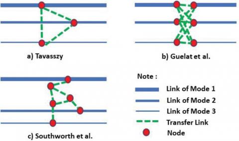
Building a transport super network means adding transfer links between modes at specific multimodal terminals, e.g., port or rail terminal. The several unimodal unite with the transfer link into a multimodal network. The mode choice becomes part of the route choice model. The multi-dimensional travel choice situation is transformed into the one-dimensional choice situation of alternative routes within the network-transshipment link proposed by Tavasszy [30], with value of cost and delay as the attribute. Guelat et al. [31] represent a more certain transfer link by adding more links in the multimodal terminal. Detailed representation of transshipment link is also proposed by Southworth and Peterson [32]. It differentiated terminal access link and transfer link in the multimodal terminal. The several terminal representations are shown in Figure 4.
Figure 4. Terminal representation (source: reference [33])
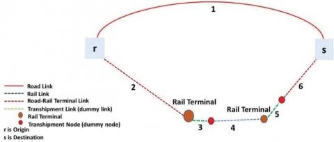
Freight network representation is described in Figure 5. Each link has a unique attribute and several transhipment links (as dummy links) are added on multimodal terminal.
Figure 5. Multimodal network representation (source: author elaboration)
Denoting k as the path in the network connecting the origin-destination pair r-s, and O–D pair belong to the set Ω, then $f_k^{r s}$ can be defined as the flow on path k connecting r-s. wais flow of goods on link a, while uais the capacity or upper limit of link a:
$w_a=\sum_r \sum_s \sum_k f_k^{r s} \delta_{a, k}^{r s} \quad \forall a \in A$ (1)
where:
$\begin{aligned} & \delta_{\mathrm{a}, \mathrm{k}}^{\mathrm{rs}}=\left\{\begin{array}{l}1 \text {, if path } \mathrm{k} \text { connecting } \mathrm{OD} \mathrm{r}-\mathrm{s} \text { using link } \mathrm{a} \\ 0, \text { otherwise }\end{array}\right. \\ & \sum_{a \in A} w_a \leq u_a, \forall a \in A \\ & \end{aligned}$
Demand associated with OD pair r-s is presented with qrs. The flow conservation and nonnegative path flow constraints are as follows:
$\begin{aligned} & q_{r s}= \sum_k f_k^{r s} \forall r, s \epsilon \Omega \\ & \mathrm{f}_{\mathrm{k}}^{\mathrm{rs}} \geq 0\end{aligned}$ (2)
Cost on link a is expressed as a generalised cost that composed of transport cost, time cost and delay cost. Further, the objective of the formulation is to minimize the total distribution cost of the system. The formulation can be described as follow:
Min Cost = C1 + C2 + C3
$C l=\sum_{a \in A}\left\{\left(P_a \times d_a \times w_a\right)+\left(H_a \times w_a\right)\right\} \times \omega_a$ (3)
$C 2=\sum_{a \in A}\left\{V O T_a\left(\frac{d_a}{v_a}+T_a\right)\right\} \times \omega_a$ (4)
$C 3=\sum_{a \in A}\left\{\operatorname{VOR}_a\left(\frac{d_a}{v_a} \times\left(1+e_a\right)\right)\right\} \times \omega_a$ (5)
where, C1 = cost related to transport cost of all links ($); C2 = cost related to time cost of all links ($); C3 = cost related to delay cost or reliability of all links ($); Pa= unit cost of link a ($/t/km); Wa= flow of commodity at link a(t); da= distance of link a (km); va= speed at link a (km/hour); VOTa= value of time at link a ($/hour); Ta= transshipment time (time at terminal) at link a (hour); VORa= value of reliability at link a ($/hour); ea= reliability at link a, describe average percentage of delayed (percentage); Ha= handling cost at terminal on link a ($/t); wa= 1, if the commodity using link a, and 0 otherwise.
Multimodal freight transport is mainly related to consolidation which a multimodal terminal has a role as a hub in the hub and spoke network. The consolidation allows cost efficiency due to the economy of scale [12]. However, this research did not consider the economics of scale in the hub node.
The selection of the best scenario relies on the Benefit-that represents efficient value and the maximum budget of IOM cost. The efficient value can be used as a parameter to assess the effective combination of development compared to initial conditions. The efficient value analysis was accounted for by considering the difference ratio between the total distribution cost without development and with development and the IOM cost. The selection also considers the maximum IOM budget. The efficient value calculation was adopted from [33] shown below:
$\max z(y)=\frac{G_o-\left(\sum_{a \in A} C_a x_a y_a\right)}{\sum_{a \in A} b_a y_a}$ (6)
Constrains:
$\sum_{a \in A} b_a y_a \leq \delta, \forall a \in A$
where, Z (y) = benefit-efficient value; G0 = total distribution cost system for all links without development for all links ($/ton); ca= total unit cost of link-a ($/ton); xa= flows on link-a (ton); ya= action implementation indicator (1 = if the development related to link a is implemented and 0 otherwise); ba= investment, operation and maintenance (IOM) cost on link-a ($).
3.5 Solution approach
The model used a bi-level approach and was solved with the Genetic Algorithm technique: An integrated freight transport network was built and equipped by origin-destination (OD) demand and attributes for each link; The lower-level optimization was performed by executing a route choice set generation to generate several alternative least-cost routes; Freight assignment and modal split were executed.
The results were freight flow and total transport cost of each link. The solution of the lower level problem was then used in the upper-level problem to obtain the cost difference between the initial condition and improved condition and later for the efficient value calculation.
Finally, the solution to the upper-level problem was used to propose the list of development actions. The combination of development included three targets, namely optimistic, moderate and pessimist targets.
Furthermore, finding an optimal combination of development and priority using the random search method under a limited budget. After the chosen combination was found and then added to the transport network, then again, Lower-level optimization of the improved or developed network was performed, the cost difference between the existing or initial condition and after development was calculated. The efficiency was obtained in addition to the mode share and the freight volume.
To support the government in prioritizing specific modes of infrastructure development (i.e., priority on the rail sector), the proposed model offers two development scenarios. In the first scenario, the model endogenously searches for the best or optimal combination of development. In contrast, in the second scenario, an intervention given on specific development combinations is set up to the model-exogenously.
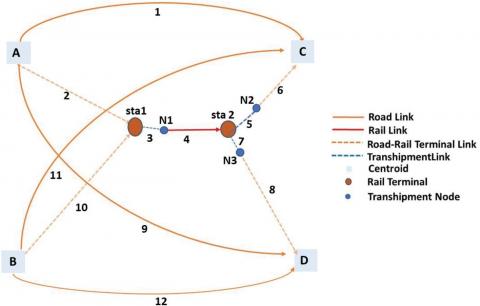
To apply the model, an illustrative example was developed. It is a small size network with dummy data. The network consists of four zone centroids with two alternative modes which are road and rail, and the latter was operated and planned in multimodal system (with road). Nodes A and B were node represent origin, while nodes C and D were destination. Each O-D pair was connected by several possible paths that consist of several links. Links was represented with number from 1 to 12. Transshipment link and transshipment node are dummy components that representing transshipment cost and time attributes between rail terminal and road, vice versa, in the multimodal rail system. Each links has cost that consist of trans-port cost, time cost and delay cost (Figure 6).
Figure 6. Sample network
Table 1. Network data
|
Link (l) |
Node start |
Node end |
Link category |
Link capacity (ton) |
Unit cost (S/km) |
Distance (km) |
|
1 |
A |
C |
Road |
200 |
0.538 |
700 |
|
2 |
A |
Sta 1 |
Road |
800 |
0.538 |
400 |
|
3 |
Sta 1 |
N1 |
Transshipment |
1,500 |
0.000 |
0 |
|
4 |
N1 |
Sta 2 |
Rail |
1,500 |
0.269 |
300 |
|
5 |
Sta 2 |
N2 |
Transshipment |
800 |
0.000 |
0 |
|
6 |
N2 |
C |
Road-station |
800 |
0.385 |
850 |
|
7 |
Sta 2 |
N3 |
Transshipment |
300 |
0.000 |
0 |
|
8 |
N3 |
D |
Road-station |
300 |
0.385 |
500 |
|
9 |
A |
D |
Road |
200 |
0.538 |
500 |
|
10 |
B |
Sta 1 |
Road-station |
800 |
0.538 |
400 |
|
11 |
B |
C |
Road |
300 |
0.538 |
900 |
|
12 |
B |
C |
Road |
300 |
0.538 |
400 |
|
Link (l) |
Speed (km/hour) |
VOT ($/hour) |
VOR ($/hour) |
Transshipment time (hour) |
Average percentage of delay (e) |
Transshipment cost ($) |
|
1 |
30 |
0.346 |
0.769 |
0 |
0.5 |
0 |
|
2 |
30 |
0.346 |
0.769 |
0 |
0.5 |
0 |
|
3 |
0 |
0.000 |
0.000 |
5 |
0.5 |
3.846 |
|
4 |
70 |
0.154 |
0.385 |
0 |
0.8 |
0 |
|
5 |
0 |
0.000 |
0.000 |
5 |
0.5 |
3.846 |
|
6 |
30 |
0.346 |
0.769 |
0 |
0.5 |
0 |
|
7 |
0 |
0.000 |
0.000 |
5 |
0.5 |
3.846 |
|
8 |
30 |
0.346 |
0.769 |
0 |
0.5 |
0 |
|
9 |
30 |
0.346 |
0.769 |
0 |
0.5 |
0 |
|
10 |
30 |
0.346 |
0.769 |
0 |
0.5 |
0 |
|
11 |
30 |
0.346 |
0.769 |
0 |
0.5 |
0 |
|
12 |
30 |
0.346 |
0.769 |
0 |
0.5 |
0 |
The network’s data is described in Table 1. For example, the link attribute consists of unit cost, link distance, speed, the value of time, reliability, transshipment time and cost, average percentage of delayed and the link’s capacity.
The time spending in the terminal consists of loading time, service time duration, and final unloading [23]. Based on reference [34], the transshipment time consists of the arrival time, service start time and departure time at the terminal. Meanwhile, in this research, the transshipment time represents the time spent in the terminal, while transfer time is represent the process before cargo unloading in the terminal.
The commodity volume from each origin and destination is described in Table 2.
Table 2. Volume from origin to destination
|
Origin |
Destination |
Volume (ton) |
|
A |
C |
500 |
|
A |
D |
500 |
|
B |
C |
300 |
|
B |
D |
900 |
The development was made in the particular links and nodes, including unimodal and multimodal links. There was three target development option: optimistic, moderate and pessimistic. The development target in the unimodal link indicates a reduction in road or rail travel time. The development of multimodal links, e.g., road-rail terminal links, indicates the reduction in travel time on that link. The optimistic target denotes travel time decreased by 50%, the average target decreased by 30%, and the pessimistic target decreased by 10%. The development at the node, such as the rail terminal, was to decrease the transshipment time. The optimistic target denotes the transshipment time decreased by 50%, the moderate target decreased by 30%, and the pessimistic target decreased by 10%. The total budget limitation was $770.000. The specific improved links and nodes are detailed in Table 3. Besides the development options, the analysis later considers two scenario conditions. It is conducted by giving intervention or prioritize on a particular node and link, such as a rail link, by setting the weight on the optimum target of development on that link or node, so the optimum target has bigger possibility to chosen as an optimal development.
Table 3. Investment, operation and maintenance cost of network development
|
No. |
Scenario of development |
IOM cost ($) |
|
1. |
Development at link 1: travel time on road decreased by 10% (Pessimistic scenario) |
53,846 |
|
2. |
Development at link 1: travel time on road decreased by 30% (Moderate scenario) |
161,538 |
|
3. |
Development at link 1: travel time on road decreased by 50% (Optimistic scenario) |
269,231 |
|
4. |
Development at link 12: travel time on road decreased by 10% (Pessimistic scenario) |
30,769,231 |
|
5. |
Development at link 12: travel time on road decreased by 30% (Moderate scenario) |
92,307,692 |
|
6. |
Development at link 12: travel time on road decreased by 50% (Optimistic scenario) |
153,846,154 |
|
7. |
Development at link 2: travel time on multimodal decreased by 10% (Pessimistic scenario) |
30,769,231 |
|
8. |
Development at link 2: travel time on multimodal decreased by 30% (Moderate scenario) |
92,307,692 |
|
9. |
Development at link 2: travel time on multimodal decreased by 50% (Optimistic scenario) |
153,846,154 |
|
10. |
Development at link 8: travel time on multimodal decreased by 10% (Pessimistic scenario) |
38,461,538 |
|
11. |
development at link 8: travel time on multimodal decreased by 30% (Moderate scenario) |
115,384,615 |
|
12. |
Development at link 8: travel time on multimodal decreased by 50% (Optimistic scenario) |
192,307,692 |
|
13. |
Development at link 4: travel time on rail decreased by 10% (Pessimistic scenario) |
32,308 |
|
14. |
Development at link 4: travel time on rail decreased by 30% (Moderate scenario) |
96,923 |
|
15. |
Development at link 4: rail travel time on rail decrease by 50% (Optimistic scenario) |
161,538 |
|
16. |
Improvement at link 3: transfer time by decreased 10% (Pessimistic scenario) |
76,923 |
|
17. |
Improvement at link 3: transfer time decreased by 30% (Moderate scenario) |
230,769 |
|
18. |
Improvement at link 3: transfer time decreased by 50% (Optimistic scenario) |
384,615 |
|
19. |
Improvement at link 7: transfer time decreased by10% (Pessimistic scenario) |
76,923 |
|
20. |
Improvement at link 7: transfer time decreased by 30% (moderate scenario) |
230,769 |
|
21. |
Improvement at link 7: transfer time decreased by 50% (Optimistic scenario) |
384,615 |
|
22. |
Development at node Sta 1: transshipment time decreased by 10% (Pessimistic scenario) |
107,692 |
|
23. |
development at node Sta 1: transshipment time decreased by 30% (Moderate scenario) |
323,077 |
|
24. |
Development at node Sta 1: transshipment time decreased by 50% (Optimistic scenario) |
538,462 |
|
25. |
Development at node Sta 2: transshipment time decreased by 10% (Pessimistic scenario) |
107,692 |
|
26. |
Development at node Sta 2: transshipment time decreased by 30% (Moderate scenario) |
323,077 |
|
27. |
Development at node Sta 2: transshipment time decreased by 50% (Optimistic scenario) |
538,462 |
Table 4. Total distribution network cost of system
|
OD |
Path |
Link |
Mode |
Volume (ton) |
Distribution Cost (million $) |
|
A-C |
A-C |
1 |
Road |
200 |
75,420 |
|
A-sta1-N1-sta2-N2-C |
2-3-4-5-6 |
Multimodal (road-rail) |
300 |
228,530 |
|
|
A-D |
A-D |
5 |
Road |
200 |
53,871 |
|
A-sta1-N1-sta2-N3-D |
2-3-4-8 |
Multimodal (road-rail) |
300 |
171,974 |
|
|
B-C |
B-C |
9 |
Road |
300 |
145,430 |
|
B-D |
B-D |
8 |
Road |
300 |
64,635 |
|
B-sta1-N1-sta2-N3-D |
10-3-4-7-8 |
Multimodal (road-rail) |
500 |
286,590 |
|
|
Total distribution cost of system |
1,026,450 |
||||
Table 5. Genetic algorithms result for 20 running
|
No run |
Total distribution cost of system |
IOM cost ($) |
Efficient value |
|
1 |
1,026,001 |
563,022 |
0.00113 |
|
2 |
1,026,407 |
624,509 |
0.00016 |
|
3 |
1,026,402 |
616,773 |
0.00023 |
|
4 |
1,025,999 |
363,012 |
0.00184 |
|
5 |
1,024,321 |
746,092 |
0.00356 |
|
6 |
1,026,416 |
558,376 |
0.00013 |
|
7 |
1,026,404 |
447,570 |
0.00027 |
|
8 |
1,026,014 |
384,579 |
0.00174 |
|
9 |
1,025,146 |
722,957 |
0.00296 |
|
10 |
1,025,158 |
538,397 |
0.00314 |
|
11 |
1,026,010 |
684,558 |
0.00225 |
|
12 |
1,026,005 |
723,022 |
0.00098 |
|
13 |
1,025,178 |
461,529 |
0.00292 |
|
14 |
1,024,321 |
693,812 |
0.00344 |
|
15 |
1,025,998 |
509,145 |
0.00150 |
|
16 |
1,025,994 |
586,045 |
0.00138 |
|
17 |
1,025,999 |
693,775 |
0.00103 |
|
18 |
1,026,009 |
689,185 |
0.00110 |
|
19 |
1,025,160 |
584,560 |
0.00298 |
|
20 |
1,026,012 |
499,952 |
0.00162 |
Figure 4. Comparison between the total distribution cost of system, total investment and efficient value
Network assignment and selection of the best development were carried out, and the result found that the total distribution network cost of system without development was $1,026,450 (Table 4). Due to the link capacity constraint, the assignment network with capacitated link and the distribution cost is shown in Table 4.
The genetic algorithm analysed the best scenario under the budget limitation. The genetic algorithm is the heuristic method; hence there is no exact result. This research used an N population of 30, while the maximum generation is 50-the running the algorithm for 20 runs. The result is revealed.
From the twenty running (Table 5 and Figure 4), the best developments were selected. It is the option with the maximum efficient value (i.e., 0.00356) and the relatively high investment (i.e., \$746.092). The total distribution cost of system was \$1,024,321. The differences between the total distribution cost of system without development and after development was \$2,129 or 0.21% (Table 7).
The best development was in the optimistic target. The development will be done at link 12 where the travel time on road decreased by 50%. The node development will be done at node Sta 1 (rail terminal) also in the optimistic target, i.e., to decrease transshipment time by 50%. Moreover, pessimistic target will be done at link 1 to reduce travel time on road by 10% (Table 6).
Table 6. Best developments
|
No. |
Best developments |
IOM cost ($) |
|
1 |
Development at link 1: travel time on road decreased by 10% (Pessimistic scenario) |
53,846 |
|
2 |
Development at link 12: travel time on road decreased by 50% (Optimistic scenario) |
153,846 |
|
3 |
Development at node Sta 1: transhipment time decreased by 50% (Optimistic scenario) |
538,462 |
|
|
Total cost of investment |
746,154 |
Table 7. Cost differences between total distribution cost of system without and after developments
|
OD |
Path |
Link |
Mode |
Vol (ton) |
Total distribution cost of system ($) |
|
|
|
Without development |
After development |
||||
|
A-C |
A-C |
1 |
Road |
200 |
75,420 |
75,416 |
|
|
A-sta1-N1sta2-N2-C |
2-3-4-5-6 |
Multimodal (road-rail) |
300 |
228,530 |
227,953 |
|
A-D |
A-D |
5 |
Road |
200 |
53,871 |
53,871 |
|
|
A-sta1-N1sta2-N3-D |
2-3-4-8 |
Multimodal (road-rail) |
300 |
171,974 |
171,397 |
|
B-C |
B-C |
9 |
Road |
300 |
145,430 |
145,430 |
|
B-D |
B-D |
8 |
Road |
300 |
64,635 |
64,625 |
|
|
B-sta1-N1sta2-N3-D |
10-3-4-7-8 |
Multimodal (road-rail) |
500 |
286,590 |
285,628 |
|
Total distribution cost |
|
|
1,026,450 |
1,024,321 |
||
Table 8. Best development with intervention on rail link
|
No. |
Best developments (intervention on rail link) |
IOM cost ($) |
|
1 |
Development at link 2: travel time on multimodal decreased by 50% (Optimistic scenario) |
153,846 |
|
2 |
Development at link 4: travel time on rail decreased by 50% (Optimistic scenario) |
161,538 |
|
3 |
Development at link 7: transfer time decreased by 10% (Pessimistic scenario) |
76,923 |
|
4 |
Development at node Sta 1: transhipment time decreased by 30% (Moderate scenario) |
323,077 |
|
|
Total cost of investment |
715,385 |
Table 9. Cost differences between existing total distribution cost and total distribution cost after developments of intervention on rail link
|
OD |
Path |
Link |
Mode |
Volume (ton) |
Total distribution cost of system ($) |
|
|
Without improvement |
After development |
|||||
|
|
A-C |
1 |
Road |
200 |
75,420 |
75,419 |
|
A-C |
A-sta1-N1sta2-N2-C |
2-3-4-5-6 |
Multimodal (road-rail) |
300 |
228,530 |
228,172 |
|
|
A-D |
5 |
Road |
200 |
53,871 |
53,871 |
|
A-D |
A-sta1-N1sta2-N3-D |
2-3-4-8 |
Multimodal (road-rail) |
300 |
171,974 |
171,616 |
|
B-C |
B-C |
9 |
Road |
300 |
145,430 |
145,429 |
|
|
B-D |
8 |
Road |
300 |
64,635 |
64,635 |
|
B-D |
B-sta1-N1-sta2-N3-D |
10-3-4-7-8 |
Multimodal (road-rail) |
500 |
286,590 |
286,010 |
|
Total distribution cost |
|
|
1,026,450 |
1,025,155 |
||
Table 10. Comparison of the total distribution cost of various scenarios of development
|
OD |
Path |
Link |
Mode |
Volume (ton) |
Total distribution cost of system without development ($) |
Total distribution cost after development ($) |
|
|
Best scenario (optimum using GA) |
Intervention on rail link |
||||||
|
|
A-E |
1 |
Road |
200 |
75,420 |
75,416 |
75,419 |
|
A-E |
A-sta1-N1- |
2-3-4- |
Multimodal |
300 |
228,530 |
227,953 |
228,172 |
|
|
sta2-N2-E |
5-6 |
rail |
|
|
|
|
|
|
A-F |
5 |
Road |
200 |
53,871 |
53,871 |
53,871 |
|
A-F |
A-sta1-N1sta2-N3-F |
2-3-4-8 |
Multimodal (road-rail) |
300 |
171,974 |
171,397 |
171,616 |
|
B-E |
B-E |
9 |
Road |
300 |
145,430 |
145,430 |
145,429 |
|
|
B-F |
8 |
Road |
300 |
64,635 |
64,625 |
64,635 |
|
B-F |
B-sta1-N1- |
10-3- |
Multimodal |
500 |
286,590 |
285,628 |
286,010 |
|
|
sta2-N3-F |
4-7-8 |
(road-rail) |
|
|
|
|
|
Total distribution cost |
1,026,450 |
1,024,321 |
1,025,155 |
||||
|
Efficient value |
|
0.00356 |
0.002 |
||||
|
Total IOM cost |
|
746,152 |
715,385 |
||||
|
% differences with initial total distribution |
|
0.21 |
0.12 |
||||
Furthermore, further development was done with the scenario to interfere the rail link. It is done to predict the effect of giving priority on rail development to the system. Link 8 was chosen to be developed with the optimistic target. The result indicated that with the IOM cost was \$715,385 (Table 8), the total distribution cost of system became \$1,025,155, and the efficient value became 0.002. While the difference with the existing distribution cost was \$1,295 or 0.12% as shown in Table 9.
Application of optimization model using GA efficiently selected the best developments. The results showed the best selection development had the highest benefit and the least distribution of the cost of the system, especially compared with the scenario development with intervention on the rail link. The intervention means prioritizing the development of the rail link by setting the weight on the optimum target of development on that link or node, so the optimum target has bigger possibility to chosen as an optimal development with travel time on the rail link decreased by 50%. The comparison result is shown in Table 10.
The model showed the efficiency in selecting the best development, especially considering the budget limitation. The conclusion drawn from the analysis is that giving priority to development on the link or node (e.g., rail link) was not given the best result. The best result found that development based on the multimodal perspectives using GA gives the best result in terms of efficient value and total distribution cost of the system.
This research is aimed to integrate the freight transport planning of multimodal transport under budget limitations on investment, operation and maintenance. The result unveiled that this model can potentially give the insight to select the best scenario of infrastructure development from the perspective of multimodal transport rather than unimodal to find the minimum distribution cost of the multimodal system. This model can produce an optimal combination of modes and the respective volumes of transportation of freight distribution system in a multimodal framework with minimum distribution cost based on the available IOM cost. This model can also find the optimal development under consideration of priority on certain modes by set up certain combination of development on the model-exogenously. The proposed model also may avoid the inefficient process of the unimodal iterative budget planning process. The proposed model can be used to integrate the planning of the transportation sub-sectors and, at the same time, develop more optimal multimodal transportation.
Further research is applying the proposed model to the entire network to test the robustness of the model. The research related to the development target at the link or node and the requirement for IOM costs also can be a potential topic.
The authors would like to thank the Indonesia Endowment Fund for education, Ministry of Finance of the Republic Indonesia, for the scholarship support to the first author of this paper.
[1] Crainic, T.G. (2003). Long-haul freight transportation. Handbook of transportation science. International Series in Operations Research & Management Science, Springer, Boston, pp. 451-516. https://doi.org/10.1007/0-306-48058-1_13
[2] SteadieSeifi, M., Dellaert, N.P., Nuijten, W., Van Woensel, T., Raoufi, R. (2014). Multimodal freight transportation planning: A literature review. European journal of operational research, 233(1): 1-15. https://doi.org/10.1016/j.ejor.2013.06.055
[3] Piccioni, C., Antomazzi, F., Musso, A. (2010). Locating combined road-railway transport terminals: an application for facility location and optimal location models. Ingegneria Ferroviaria, 65(7-8): 625-649.
[4] Kumar, A., Anbanandam, R. (2019). Multimodal freight transportation strategic network design for sustainable supply chain: an or prospective literature review. International Journal of System Dynamics Applications (IJSDA), 8(2): 19-35. https://doi.org/10.4018/IJSDA.2019040102
[5] Lubis, H.R., Prasetyo, L.B.B., Samuel, E.L.I.M. (2003). Multimodal freight transport network planning. Journal of the Eastern Asia Society for Transportation Studies.
[6] Mostert, M.A.R.T.I.N.E., Caris, A., Limbourg, S.A.B.I. N.E. (2017). Road and intermodal transport performance: the impact of operational costs and air pollution external costs. Research in Transportation Business & Management, 23: 75-85. https://doi.org/10.1016/j.rtbm.2017.02.004
[7] Tavasszy, L., De Jong, G. (2013). Modelling Freight Transport. Elsevier.
[8] Kramarz, M., Dohn, K., Przybylska, E., Knop, L. (2020). Scenarios for the development of multimodal transport in the TRITIA cross-border area. Sustainability, 12(17): 7021. https://doi.org/10.3390/su12177021
[9] Perhubungan, K. (2019). Rencana induk transportasi nasional. Kementerian Perhubungan: Jakarta.
[10] Guglielminetti, P., Piccioni, C., Fusco, G., Licciardello, R., Musso, A. (2017). Rail freight network in Europe: Opportunities provided by re-launching the single wagonload system. Transportation Research Procedia, 25: 5185-5204. https://doi.org/10.1016/j.trpro.2018.02.047
[11] Crainic, T.G., Florian, M. (2008). National planning models and instruments. INFOR: Information Systems and Operational Research, 46(4): 299-308. https://doi.org/10.3138/infor.46.4.299
[12] Racunica, I., Wynter, L. (2005). Optimal location of intermodal freight hubs. Transportation Research Part B: Methodological, 39(5): 453-477. https://doi.org/10.1016/j.trb.2004.07.001
[13] Hanaoka, S., Regmi, M.B. (2011). Promoting intermodal freight transport through the development of dry ports in Asia: An environmental perspective. Iatss Research, 35(1): 16-23. https://doi.org/10.1016/j.iatssr.2011.06.001
[14] Zhang, M., Janic, M., Tavasszy, L.A. (2015). A freight transport optimization model for integrated network, service, and policy design. Transportation Research Part E: Logistics and Transportation Review, 77: 61-76. https://doi.org/10.1016/j.tre.2015.02.013
[15] Chang, T.S. (2008). Best routes selection in international intermodal networks. Computers & operations research, 35(9): 2877-2891. https://doi.org/10.1016/j.cor.2006.12.025
[16] Yamada, T., Russ, B.F., Castro, J., Taniguchi, E. (2009). Designing multimodal freight transport networks: A heuristic approach and applications. Transportation science, 43(2): 129-143. https://doi.org/10.1287/trsc.1080.0250
[17] Sjafruddin, A., Lubis, H.A.R.S., Frazila, R.B., Dharmowijoyo, D.B. (2009). Policy Evaluation of Multimodal Transportation Network, the Case of Inter Island Freight Transportation in Indonesia. In Proceedings of the Eastern Asia Society for Transportation Studies, 7: 142-142. https://doi.org/10.11175/eastpro.2009.0.142.0
[18] Beuthe, M., Degrandsart, F., Geerts, J.F., Jourquin, B. (2002). External costs of the Belgian interurban freight traffic: A network analysis of their internalisation. Transportation Research Part D: Transport and Environment, 7(4): 285-301. https://doi.org/10.1016/S1361-9209(01)00025-6
[19] Geerts, J.F., Jourquin, B., Luc, L.U.C. (2001). Freight transportation planning on the European multimodal network. EJTIR, 1(1): 91-106.
[20] Limbourg, S., Jourquin, B. (2009). Optimal rail-road container terminal locations on the European network. Transportation Research Part E: Logistics and Transportation Review, 45(4): 551-563. https://doi.org/10.1016/j.tre.2008.12.003
[21] Jonkeren, O., Jourquin, B., Rietveld, P. (2011). Modal-split effects of climate change: The effect of low water levels on the competitive position of inland waterway transport in the river Rhine area. Transportation Research Part A: Policy and Practice, 45(10): 1007-1019. https://doi.org/10.1016/j.tra.2009.01.004
[22] Jourquin, B., Iassinovskaia, G., Lechien, J., Pinna, J., Usai, F. (2009). Lines and services in a regional multi-modal transport model: The case of the regional express network around Brussels. Proceedings of the Bivec-Gibet Transport Research Day, 839-856.
[23] Bilegan, I.C., Crainic, T.G., Wang, Y. (2022). Scheduled service network design with revenue management considerations and an intermodal barge transportation illustration. European Journal of Operational Research, 300(1): 164-177. https://doi.org/10.1016/j.ejor.2021.07.032
[24] Cascetta, E. (2013). Transportation systems engineering: theory and methods. Springer Science & Business Media.
[25] Grosso, M. (2011). Variables Influencing Transport Mode Choice: A Generalized Cost Approach. Proceedings XIII Riunione Scientifica Società Italiana dei Trasporti e della Logistica, Messina.
[26] De Jong, G., Kouwenhoven, M., Kroes, E., Rietveld, P., Warffemius, P. (2009). Preliminary monetary values for the reliability of travel times in freight transport. European Journal of Transport and Infrastructure Research, 9(2): 83-99. https://doi.org/10.18757/ejtir.2009.9.2.3291
[27] Feo-Valero, M., García-Menéndez, L., Garrido-Hidalgo, R. (2011). Valuing freight transport time using transport demand modelling: a bibliographical review. Transport Reviews, 31(5): 625-651. https://doi.org/10.1080/01441647.2011.564330
[28] Shams, K., Jin, X., Fitzgerald, R., Asgari, H., Hossan, M.S. (2017). Value of reliability for road freight transportation: evidence from a stated preference survey in Florida. Transportation Research Record, 2610(1): 35-43. https://doi.org/10.3141/2610-05
[29] Sheffi, Y. (1985). Urban transportation networks. Prentice-Hall, Englewood Cliffs, NJ.
[30] Tavasszy, L. (1996). Modeling European freight transport network. The Netherlands Research School for Transport, infrastructure and Logistics.
[31] Guelat, J., Florian, M., Crainic, T.G. (1990). A multimode multiproduct network assignment model for strategic planning of freight flows. Transportation science, 24(1): 25-39. https://doi.org/10.1287/trsc.24.1.25
[32] Southworth, F., Peterson, B.E. (2000). Intermodal and international freight network modeling. Transportation Research Part C: Emerging Technologies, 8(1-6): 147-166. https://doi.org/10.1016/S0968-090X(00)00004-8
[33] Russ, B.F., yamada, T., Castro, J.T., Yasukawa, H. (2005). Optimising the design of multimodal freight transport network in Indonesia. Journal of the Eastern Asia Society for Transportation Studies, 6: 2894-2907. https://doi.org/10.11175/easts.6.2894
[34] Zhang, Y., Atasoy, B., Souravlias, D., Negenborn, R.R. (2020). Pickup and delivery problem with transshipment for inland waterway transport. In Computational Logistics: 11th International Conference, ICCL 2020, Enschede, pp. 18-35. 10.1007/978-3-030-59747-4_2