Antonio Di Pietro*![]() | Luigi De Dominicis
| Luigi De Dominicis![]() | Giuseppe A. Marzo
| Giuseppe A. Marzo![]() | Arnab Paul
| Arnab Paul![]() | Nicola Ranieri
| Nicola Ranieri![]() | Vittorio Rosato
| Vittorio Rosato![]()
© 2023 IIETA. This article is published by IIETA and is licensed under the CC BY 4.0 license (http://creativecommons.org/licenses/by/4.0/).
OPEN ACCESS
An optimized algorithm for allowing the autonomous search of a radioactive source has been designed and implemented as a firmware on an UAV. The algorithm has been designed to comply with several constraints imposed by UAV and by the radiation sensor, in terms of electrical autonomy and time duration of the measurement process. The algorithm implements a gradient descent strategy which allows to recover, with a good spatial resolution, the radiation source whose position and type (i.e., activity) is not a priori known. The algorithm was validated through a Monte Carlo simulation and incorporates problem’s constraints regarding the search area. Simulation results show that the UAV is able to appropriately locate the source location with high success rate during a single UAV mission and to estimate the total time of the operation.
UAV, physical security, radiological survey, gradient descent algorithm, firmware, monte carlo simulation
In radiological and nuclear (RN) emergencies, radiation mapping is a process adopted to locate and identify the radioactive source(s) in specific areas and to evaluate their activity. So far, this task has been largely accomplished mobilizing manned aircrafts equipped with bulky and high-weight radiation detectors [1]. This solution, if from one hand guarantees the coverage of large areas during the survey, on the other generates data with low spatial resolution that in some cases not always up to solve positively the mission tasks. This is due to the altitude at which the manned aircraft operates and to the radiation detectors field of view (FOV). For instance, for a flight altitude of 150 m and a detector FOV of 56° (typical of scintillators) the resolution is around 239 m.
Nowadays, thanks to the rapid and growing advancements in capabilities, unmanned aircraft systems (UAS/drones), once equipped with radiation detectors, can largely improve spatial resolution on the ground by using low altitude fly-over and by doing an appropriate trade-off between ground resolution and total scanned surfaces. It turns out that the use of UAS in RN emergencies is a subject of growing interest for supporting First Responders (FR) when they are called to perform complex tasks under harsh operating conditions. Drones can provide reliable support in their work and the operational concept is that, when a radiation emergency occurs, FRs deploy the UAV to determine the location of radiation sources, to survey the area and to generate a map of radiation levels and finalized at planning and implementation of the appropriate response plan.
Nevertheless, there are many difficulties to solve to make radiation detection by UAS/drones a performing practice in RN emergencies. Among them the main difficulties, as indicated in the paper, are related to constraints imposed by the current UAV technologies for civil purposes ((a) in the following) and by a further self-imposed constraint ((b) in the following):
(a) The small payload allowed for a UAV complies the use of light radiation counter which inhomogeneous sensibilities as a function of the radiation energy;
(b) The limit of being able to make a detection in the time span of a single mission.
The development of low weight radiation detectors and of appropriate flight plans are common to all possible intervention scenarios. In particular, radiological survey mission scenarios can include the following issues: (i) source seeking and localization; (ii) survey of radionuclides deposited on the ground; (iii) radioactive plume tracking; (iv) onsite survey in case of a nuclear/radiological incident; (v) internal survey of a reactor building; (vi) source search after an information alert and (vii) accident involving a vehicle carrying radioactive material on city road/highway.
These scenarios can be implemented through manual or autonomous operations. In the first case, a pilot or an observer in contact with the pilot, should keep the UAS within visual line of sight (VLOS) during flight. The latter include semi-autonomous or fully-autonomous operations where the Unmanned Aerial Vehicles (UAV) adaptively defines its route without the pilot and/or beyond the visual line of site (BVLOS) on the bases of some specific input provided by on-board devices (e.g., sensors). The resulting radiological survey can be represented by a gamma-dos rate map that shows detected radiation hot spots, possibly along with isotopic data.
Typical parameters that should be considered when planning the mentioned scenarios are listed in the following:
In this paper, we investigate how a proper set of the mentioned parameters could be combined and applied in autonomous operations dealing with source seeking and localization, in order to reduce the total time of the operation. However, the weight of these parameter strictly depends on the specific operation plan and cannot be specified in general. Some parameters are also dependent on each other and can lead to conflicting situations: for example, in the case of a high source, too low a flight height will cause sensor saturation while too high a height will cause only background radiation to be detected.
In particular, the addressed problem is to allow the UAV to detect the presence of a radiation source hidden in the ground by using a GM detector and without any form of visual inspection provided by cameras. Visual inspection of photos produced by cameras will require a complete detailed photography of the suspected area, but does not always guarantee simplicity to have a source being detected successfully. Moreover, that process must be finally verified through an open-eye inspection, involving investigations with time complexity up to large degrees. Highlighting the fact that visual inspection includes direct physical exposure of a human operator to radiation for a long period of time can be hazardous to the operator’s life.
The proposed approach has been validated by using a Monte Carlo simulation [2] which allows to emulate the path followed by the UAV and to measure the total time required for the UAV to find a radiation source, the resulting accuracy (in terms of the distance between the predicted and the real source location and the difference between the predicted and the real source activity) in an open field. In particular, a background radiation and the position of the source are stochastically determined at each simulation (what does it mean ???). In this context, a generic simulated flight plan consists of a sequence of points at a fixed altitude where a radiation measurement is simulated at each point to emulate the acquisition of a GM detector. In addition, a search strategy was implemented with the aim of avoiding an exhaustive scan of the considered area so as to reduce the total operation time. Indeed, the sequence of measurement points is produced by an optimized procedure based on the Gradient Descent (GD) algorithm [3], which allows to minimize a specific function of the radiation intensity by iteratively moving in the direction of steepest descent as defined by the negative of the gradient. The approach models the physical laws of gamma radiation propagation so that the radiation intensity decreases by the square of the distance from the source, according the inverse square law for radiation. In general, the model integrates: (i) radiologic assumptions (type of source, intensity, background radiation, duration of one GM detector measurement); (ii) geometric assumptions of the search area (extent, UAV altitude, cell size) and (iii) algorithmic assumptions (GD activation properties, maximum moves allowed).
This work follows a practical experience of deployment of a system integrating a commercial UAS (DJI Inspire 2) equipped with a GM detector capable of recording radioactive decay energies and integrated into a Raspberry device to control and transmits data to a ground station [4]. This system was applied to a source seeking and localization mission to implement an optimized strategy with the aim of avoiding an exhaustive scan of the predetermined area so as to reduce the total operation time. In the present paper, details of such procedure are described and validated through simulation.
The described system is part of the actions of the EU INCLUDING project whose main objective is to enhance practical knowledge to boost a European sustainable training and development framework for practitioners in the RN Security sector [4]. The results presented in this work want to validate the search procedure and drive next investments in RN emergencies where the deployment of UAV could contribute to more efficient mission objectives.
This paper is structured as follows. Section 2 describes related work in the area. Section 3 presents radiologic preliminaries. Section 4 focuses on the model implementation properties and discusses model results. Finally, in Section 5, some conclusions and ideas for future works are drawn.
The following works are related to reference missions where small battery powered UAVs have been used.
Molnar et al. [5] used a small-sized drone to produce a gamma radiation distribution according to a two-step procedure. In the first one they employed aerial photography to acquire overlapping photographs required to generate an orthophoto and in the second one they employed a GM tube to evaluate the radiation field according to a shared grid. Then, they combined the orthophoto with the radiation map to verify in a visual way that the source could be localized within a certain error. However, this approach required a complete scan of the area.
Gordon et al. [6] used a heavy UAV (2005 Yamaha RMAX model: L17-2) equipped with a NaI (Tl) radiation detector for radiation mapping and, a two-camera stereo boom for imaging terrestrial topology. They also used an UGV DySMAC TURTLE (built as Terrestrial Unmanned Robots for Teamed Learning and Exploration) equipped with RSI 701 radiation detector and a Velodyne HDL32-E LiDAR. The UGV used the orthophoto, DEM and segmentation produced by the UAV to scan an area of interest. The attached LiDAR would secure obstacle-free paths for the UGV. The procedure is only off-line and requires a complete scan of the area. In addition, computational time is high.
Bai et al. [7] developed a monitoring system consisting of a quadrotor DJI Matrice 100 drone hovering at 10 m above ground, equipped with an ARD100 radiation detection sensor. The sensor uses a low range NDL-11 silicon photodetector + CsI (Tl) scintillator. They conducted the field experiment on a rectangular area of 30×25 m, with 241Am radioactive sources of radioactivity were selected within 3.7×10⁹ Bq, being randomly placed within the selected area. Three different algorithms for radioactive source search were proposed and theoretically compared in terms of search-time complexity. These algorithms implement a complete scan of the area, a binary search and a successive approximation respectively and the required computational time is also discussed. Compared to the first two algorithms, the third one requires the radioactive source with higher activity. Thus, the obvious change of dose rate can be detected even at the boundaries of the 30×25 m field; in case of a weak source that might not be detected, the procedure requires a complete scan of the area until a significant dose intensity is found.
Steinhäusler et al. [8] produced a report about the radiation monitoring around the Fukushima Daiichi Nuclear Power Plant [9] and the search of radioactive debris from the Russian satellite Cosmos 954 (Operation "Morning Light") [10]. In the first scenarios, an AUH (RMAX G1) unmanned helicopter manufactured with three LaBr3: Ce scintillation detectors capable of creating an Aerial Radiation Measurement System (ARMS) was deployed in the Fukushima Daiichi Nuclear Power Plant. In reference [11], the authors described an airborne with a spectrometer consisting of sodium iodide detector for the radioactive debris search. Research studies mentioned on references [9, 11] both implemented a complete scan of the areas before concluding with a map depicting the radiation intensities inside the zones.
In the framework of the Action Plan on Nuclear Safety [12], the IAEA has assisted Fukushima Prefecture through two consecutive cooperation projects from 2012 to 2020 to provide: (a) a complete UAV-based instrumentation system for radiation measurements developed and built at the IAEA Nuclear Science and Instrumentation Laboratory (NSIL), and (b) a post-measurement analysis and interpretation methodology as well as training personnel on how to apply the UAV and its instrumentation system as well as on how to use the software for obtaining and interpreting data.
Lim et al. [13] demonstrated how the delivery scheduling of an UAV can be optimized studying the Payload-induced Battery Consumption Rates. The status of the art detailed by Steinhäusler et al. [8] in their report considers only small battery powered (capable of low flying) UAVs with payload high enough to carry out radiation measurements. But the optimization algorithm developed by us later in this paper never rejects the fact of capability of implementation even with petrol powered hybrid drones.
Since time can be very costly in RN emergency situations, the development in the rescue operation technologies is always aimed at optimizing the time complexity. In our work, the optimization has been done by pushing the system to avoid complete scanning of the considered terrestrial area but successfully produce mapping of radioactive zones in a reduced interval of time.
3.1 Search area assumptions
In this Section, geometric properties of the search area will be described. The search area is defined as the region of a space where the UAV is supposed to flight to implement the search and localization operation.
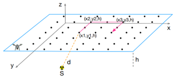
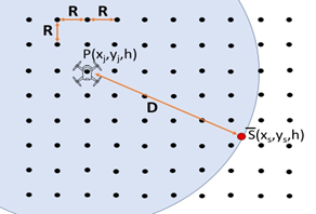
Let Ω be a cartesian space with Ω=ℝ3. A search area β is defined as a rectangle of dimensions L×W that lies on plan α as depicted in Figures 1 and 2. The search area β consists of several adjacent square-shaped cells ciof size R s.t.: L=Xmax ·R, W=Ymax·R with Xmax, Ymax, R∈ℝ, 1≤ci≤Xmax+Ymax.
Figure 1. 3D-view of the UAV search area
Figure 2. Top view of the search area
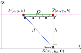
Let S∈Ω be a source located in the ground s.t. S=(xs,ys,0) and S̅=(xs, ys, h) the projection on β. A generic route performed by the UAV consists of an ordered sequence $\bar{\Gamma}_i^K$ of K points at a fixed altitude h that lie on A:
$\Gamma_i^K$={P(xj, yj, h)} (1)
with, j∈{1 ,.., K}, $\left|\Gamma_i^K\right|$=K. Thus, the radial distances d and D of a generic point P(xj, yj, h) from S and S̅ are respectively:
d=d(P,S)=|P–S| (2)
D=d(P,S̅)=|P−S̅| (3)
Knowing d and H, we could obtain D (from Pythagoras’ theorem):
$D=\sqrt{d^2+h^2}$ (4)
Table 1 summarizes the parameters used to model the search area.
Table 1. Geometric properties of the search area
|
SYMBOL |
DESCRIPTION |
UM |
|
L |
Length of the search area |
m |
|
W |
Width of the search area |
m |
|
h |
Altitude of search area above the ground |
m |
|
S |
Source location on the ground |
- |
|
Xmax |
Number of x cells of the search area |
- |
|
Ymax |
Number of y cells of the search area |
- |
|
R |
Distance between two adjacent cells |
m |
|
D |
Radial distance of P(xj,yj,h) from S¯(xs,ys,h) |
m |
|
d |
Distance of P(xj,yj,h) from S(xs,ys,0) |
m |
3.2 Radiologic properties
Based on the above geometric assumptions and the radiologic quantities presented in Appendix A, in this Section, the radiologic properties we considered for the model are presented and related to the position of the UAV in the search area β (Figure 3).
Figure 3. Horizontal view of the search area
In particular, the model allows to simulate the search operation of different gamma sources with specific activity A (in MBq). Indeed, considering a specific source with activity A, and a quality factor q (see Appendix A.5), the effective dose E, that is calculated by the model and specified in Eq. (4), is dependent on the distance d only, as specified in the following:
$E=E(d) \propto \frac{1}{d^2}$ (5)
Let us assume:
Definition 1. (Radial Radius of influence). The radius of influence d̅ is the maximum radial distance |P–S| between the UAV position P and S s.t.:
E(d̅)=E̅≥B (6)
Definition 2. (Planar Radius of influence). The planar radius of influence D̅ is the maximum distance |P−S̅| between the UAV position P and S̅ when d=d̅.
In other words, the variable D̅ defines the maximum radius of a circle, called coverage area, where the GM detector can reveal a source. The higher D̅, the more extensive is the area where the GM detector can reveal sources.
Table 2 shows the expected effective doses E for different values of d for 60Co isotope. For example, let us consider a background radiation value B=0.17 and a GM detector at an altitude h=10 and apply the above definitions. Indeed, the last row of Table 2 show the value of the radial d̅ and planar D̅ radius of influence respectively. Thus, the value of D̅ is an indicator of the density of measurements that are required by the GM detector to reveal sources in the area of interest.
Table 2. Expected effective dose values evaluated at different radial distances d for Isotope=60Co at altitude h=10
|
Radial distance d |
Planar distance D |
Dose E |
|
10 |
0 |
3.58 |
|
14.1 |
10 |
1.79 |
|
22.4 |
20 |
0.72 |
|
26.9 |
25 |
0.49 |
|
31.6 |
30 |
0.36 |
|
46.1 |
45 |
0.17 |
3.3 Algorithmic assumptions
Definition 3. (Sample distance). The sample distance Fk+1 is defined as the distance among two points Pk+1 and Pk, s.t.:
Fk+1=|Pk+1−Pk| (7)
Definition 4. (Total duration of the operation). The total duration of the operation Top is defined as the duration (in seconds) required to one simulated procedure to find the source, s.t.:
Top=K·∆Tcoll (8)
with, K≥1 is the number of points visited by the UAV and ∆Tcollis the time required by the GM detector for one measurement point. [In practical applications, this parameter may include also the time required to transmit the value to a ground station device where the proposing algorithm executes and the UAV position is calculated and sent to the UAV.] It is worth noting that each point is generated at a time by the proposed automated procedure and a measurement is acquired after the UAV reaches the new position. Thus, in detection time depends on (a) quality of the instruments used; (b) data processing time; (c) activity of the source and (d) detector type.
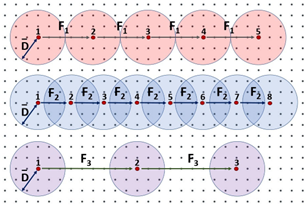
Figure 4. Possible configuration of sample distance F
Figure 4 shows three significant values of F that influence the total coverage area performed by the UAV in a search operation. In particular, assuming F=F2≈2·D̅, a high coverage area will be monitored; however, this will increase the average time T of the operation because the UAV will visit a higher number of points. By choosing F=F1<<2·D̅ and F=F3>>2·D̅, no (a complete) overlapping of the influence areas will be implemented. This will decrease the average time T of the operation; however, the success rate of finding the source within the considered interval will be lower. However, the scope of this study is not to find an optimal F-value but to show the dependency of the parameters introduced and how a proper set of them will lead to the source localization.
Table 3. Algorithmic assumptions
|
SYMBOL |
DESCRIPTION |
UM |
|
B |
Background radiation |
µSv/h |
|
N |
Number of cells between two measurements |
- |
|
F |
Sample distance |
m |
|
η |
Learning rate |
m |
|
∆Tcoll |
Measurement collection time of the GM detector |
sec |
3.4 UAV autonomous procedure
The proposed procedure for autonomous search and localization of a source is based on two consecutive phases with different paths: (i) Phase 1: Snail-like path and (ii) Phase 2: Optimized path.
Let us generalize the sequence of points Γ=ΓK of a generic mission as defined in (1) to include the two above mentions UAV paths:
$\Gamma=\bar{\Gamma} \cup \widehat{\Gamma} \cup \dot{\Gamma}$ (9)
where,
Considering that the position of the source is not known at the beginning of any search, Phase 1 performs a snail-like path until a radiation measurement is higher than the expected radiation background B, an optimized procedure will start to continue the search in a smaller area. However, in case the search area in the snail-like path has a high value of F, all the search area will be visited in Phase 1; in this case, the Phase 2 will not execute.
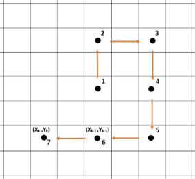
Figure 5. An example of snail-like path
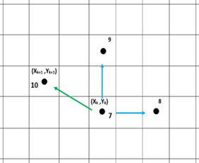
Figure 6. An example of an optimized path
3.4.1 Snail-like path
This phase is performed at the beginning of the procedure and consists of a set of points at a fixed altitude h defined by $\bar{\Gamma}$. The length F of each step constant in Phase 1 and is defined s:F=N·R with N∈Z being a constant value with N≥1, s.t.:
|Pj+1−Pj|=F (10)
with, 0≤j≤σ, Pj+1,Pj∈$\bar{\Gamma}$. Figure 5 represents an example of the points that are generated in this Phase according to a snail-like path.
3.4.2 Optimized path
In order to increase the fitting in a specific area, Phase 2 employs "Gradient-Descent (GD hereafter) technique (also often called steepest-descent) that is an iterative first-order optimization algorithm used to find a local minimum/maximum of a given function. This method is commonly used in machine learning (ML) to minimize a cost/loss function (e.g., in a linear regression).
In order to find the minimum of a continuously differentiable function f(x), the general form of the Gradient-Descent algorithm is given as:
$\begin{gathered}x_1=x_0-\eta \cdot \nabla f\left(x_0\right) \\ x_2=x_1-\eta \cdot \nabla f\left(x_1\right) \\ \cdots \\ x_{n+1}=x_n-\eta \cdot \nabla f\left(x_n\right)\end{gathered}$ (11)
where, η is the learning-rate, t that determines the step size at each iteration. In our case, the objective is to maximize the function E(x, y, z) representing the radiation intensities on the Cartesian space P(x, y, z).
Figure 6 shows an example of the application of GD algorithm that follows a snail-like path depicted in Figure 5. In particular, at step 10 of the procedure, we have:
It can be noticed by the code, that the sample distance F it remains constant in Phase 1 whereas it varies in Phase 2 according to the learning rate η. The value set for η is purely empirical, which we have decided according to multiple simulation results. Any value higher than the one considered (η=1) will increase the number of samplings before reaching the maximum; on the other hand for lower values, may lead to simulations missing the maximum. In other words, in Phase 2, the algorithm adaptively tries to increase the density of the number of measurements to find a maximum of the function E.
3.4.3 Pseudocode
Pseudocode 1 describes the algorithm of a generic iteration of the Monte Carlo simulation.
|
Pseudocode 1. General structure of the algorithm |
|
1: Pxy=Pxy−mink[Pxk]←∀ x=0, 1, 2, ..., n; 2: Pxy=Pxy−mink[Pky]←∀ y=0, 1, 2, ..., m; 3: P=Φ; 4: 0<M<Mmax=moves; 5: Tmax=f(Mmax); 6: N=1, 2, 3,... ← : (Pxy +N) ∈P; 7: 0<E < Emax = dose at (x,y); 8: G=1, 2, 3, ... ←: G≤N; 9: η = empirical value; 10: Gradient of dose variation along x−axis=∇x; 11: Gradient of dose variation along y−axis=∇y; 12: if |P|< n & m && M < Mmax && Tmax=false then 13: Start measure E at (n/2, m/2); 14: Fk+1=Fk 15: Continue in snail-like path [: next measure at +N]; 16: if Tmax=true then 17: Do not enter in any other loop; 18: end if 19: if E>B then 20: initial G= empirical value; 21: loop 22: function GRADIENT-DESCENT (Pseudocode 2) 23: end function 24: end loop 25: end if 26: end if |
|
Pseudocode 2. Pseudocode of the GRADIENTDESCENT FUNCTION |
|
1: while |P|< n & m && M < Mmax && Tmax = false do 2: Measure E at (x+G, y)= a; 3: Measure E at (x, y+G)= b; 4: ∇x = ((a − E)/G) · η; 5: ∇y = ((b − E)/G) · η; 6: F(x)k+1 = F(x)k − |∇x|; 7: F(y)k+1 = F(y)k − |∇y|; 8: if ∇x ≥ 0 then 9: xk+1 = xk+ F(x)k+1; 10: else 11: xk+1 = xk− F(x)k+1; 12: end if 13: if ∇y≥0 then 14: yk+1=yk+F(y)k+1; 15: else 16: yk+1=yk−F(y)k+1; 17: end if 18: if Tmax = true then 19: Do not enter in any other loop; 20: end if 21: end while |
After variable setting, the algorithm starts the snail-like path (line number 15) at altitude h. Line number 20 indicates that the GD algorithm will be executed if the effective dose E is greater than the background radiation B. The GD algorithm is described in Pseudocode 2.
Based on Figure 6, in the following we analyze the mail algorithm steps assuming that the GD has been triggered at point $\dot{P}_{7}$:
(1) two radiologic measurements are performed and two control points $\hat{P}_8^7$ and $\hat{P}_9^7$ are produced s.t. (line numbers 2-3 in Pseudocode 2);
(2) a new step size D8 is calculated through the gradient of function f(·) along x and y axis (line numbers 6-7 in Pseudocode 2) where η gives a doping effect to the reduction of the step size while approaching the function’s maximum.
$\nabla f\left(\dot{P}_7\right)=\left(\left(f\left(\dot{P}_8^7\right)-f\left(\dot{P}_7\right)\right) / G\right) \cdot \eta$ (12)
$\nabla f\left(\dot{P}_8\right)=\left(\left(f\left(\dot{P}_9^7\right)-f\left(\dot{P}_7\right)\right) / G\right) \cdot \eta$ (13)
$F_{10}=F_7-\left|\nabla f\left(\hat{P}_8^7\right)\right|$ (14)
$F_{10}=F_7-\left|\nabla f\left(\hat{P}_9^7\right)\right|$ (15)
(3) a new point P10 (P10∈$\dot{\Gamma}_i$) is calculated and visited (line numbers 9-16 in Pseudocode 2) where +(−) applies when ∇x≥0 (∇y≥0) respectively.
x10=x7±F10 (16)
y10=y7±F10 (17)
The GD algorithm terminates when a maximum dose value $\bar{E}$=Pµis reached after 5 consecutive increasing values of E. The termination condition called exit_cond is defined as follows:
exit_cond : E(P˙µ)≥E(P˙µ−i) (18)
where i=1, ..., 5.
Figure 7. Path tracking of the UAV from a simulation
Figure 7 depicts the result of one simulation consisting of 45 points in a search a L x W field with L=150 and W=150. In this particular execution, the GD algorithm was triggered at point P20.
4.1 Monte Carlo simulation
In order to estimate the overall efficiency of the algorithm, we carried out several Monte Carlo simulations for estimating the algorithm performances. In addition to the search area and algorithmic properties reported in Tables 1 and 3, the following properties of the implemented search algorithm should be known in advance: (a) the average number of measurements required to discover the source location; (b) the accuracy in locating the xy coordinates of the radiation source in the ground, as a function of the UAV mission height; (c) the total time required to complete the mission within the maximum time; (d) the fraction of the total electrical autonomy deployed for the mission.
One simulation consists of Ns=10000 executions where the source location changes at each iteration. In particular, a radiation source is randomly located in the search area at altitude h=0 and the specific effective dose is calculated on the search area. This calculation considers the radiation associated to the specific source and the background radiation B, expressed as a stochastic value. Then, according to the selected parameters the path of the UAV is simulated and a set of output parameters are calculated.
4.2 Simulation setup
Six scenarios were executed with preassigned values for our assumed parameters (Tables 4 and 5).
Table 4. Common simulation properties for scenarios 1-6
|
Symbol |
q |
Q |
γ |
R |
A |
L |
W |
η |
ζ |
Mmax |
∆Tcoll |
|
Value |
1.17 |
1 |
8.5×10⁻¹⁷ |
1 |
103 |
100 |
100 |
10-3 |
≤0.09 |
300 |
20 |
Table 5. Specific simulation properties for scenarios 1-6
|
SCENARIOS |
1 |
2 |
3 |
4 |
5 |
6 |
|
h |
20 |
15 |
10 |
20 |
15 |
10 |
|
F |
10 |
10 |
10 |
15 |
45 |
5 |
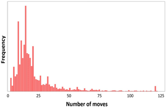
Figure 8. Histogram generated from the data of simulation results for scenario 3
In particular, we considered a 60Co isotope at different values of altitude h and sample distance F respectively. Based on practical experiences of GM detector measurements, we defined an appropriate value range for the altitude h. That includes an upper limit to avoid faint source detection of background radiation and a lower limit to avoid saturation of the GM detector. Regarding the sample distance F, different values of the distance value F were chosen to evaluate the effect of different rate of measurements. Based on past practical experiences, we considered ∆Tcoll=20 sec as the measurement collection time including also the transmission time required from the drone to the ground station.
In order to model the success rate of one execution of the algorithm, we defined Mmax as a maximum number of moves allowed. In case a source is not found within the Mmax moves or the total area is visited in Phase 1, then the execution is considered failed; otherwise, the source is found.
Finally, the ζ value was defined to consider the noise phenomenon present in the radiation intensity measurement (expressed as µSv/h).
4.3 Simulation results
Simulation results are shown in Table 6 whereas Figure 8 shows a histogram of the statistical data obtained from scenario 3.
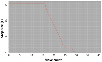
Figure 9. Evolution of the step size through Phase 1 and 2 during scenario 3
Table 6. Results obtained from simulations presented in Table 5
|
SCENARIOS → |
1 |
2 |
3 |
4 |
5 |
6 |
|
Success rate |
94% |
95% |
96% |
91% |
61% |
86% |
|
Max. moves |
122 |
122 |
122 |
123 |
18 |
301 |
|
Min. moves |
2 |
2 |
2 |
2 |
2 |
2 |
|
Moves’ Sum |
209822 |
212123 |
218975 |
358412 |
139292 |
622841 |
|
Error-margin mean |
2.64 m |
2.34 m |
2.22 m |
2.61 m |
2.33 m |
2.25 m |
|
D̅ |
41.30 |
43.37 |
44.79 |
41.31 |
43.35 |
44.76 |
|
∆D̅ |
2.91 |
2.47 |
2.27 |
2.92 |
2.46 |
2.26 |
|
Geomtric Mean |
15.52 |
15.98 |
16.59 |
27.54 |
13.37 |
40.21 |
|
80’ Percentile |
27 |
26 |
28 |
51 |
16 |
105 |
|
Mean |
20.98 |
21.21 |
21.90 |
35.84 |
13.93 |
62.28 |
|
Variance |
385.45 |
398.61 |
402.33 |
703.59 |
11.03 |
2933.23 |
|
Stnd. Dev. |
19.63 |
19.97 |
20.06 |
26.53 |
3.32 |
54.16 |
|
Skewness |
2.56 |
2.73 |
2.67 |
1.42 |
-1.25 |
1.20 |
|
Kurtosis |
7.40 |
8.23 |
8.04 |
1.73 |
0.85 |
1.13 |
For each scenario, the error margin of the estimated source location was calculated by comparing the known position with the estimated value. This parameter was used to infer, with a certain error (∆D̅), the planar radial of influence D.
It can be noticed that the success rate has slightly improved from scenario 1 to 3. This can be explained by a lower altitude h chosen that increase the value of the planar radial of influence D. This will increase the overlap rate of the coverage areas i.e., the capacity of the GM detector to reveal the source. This behavior can be noticed by a higher value of the average duration of the search operation in Scenario 3 (21,9 s). Table 9 shows the trend of F in scenario 3: it can be noticed that this value decreases during Phase 2 to increase the number of points in a limited area of search. Finally, scenario 5 exhibits the lower average duration of the search operation. However, it has the lower success rate (61%). This can be explained by the high value of the sample distance F that reduce the number of total measurements; in particular, in some cases, the Phase 1 is executed only with a total scan of the area implemented in Phase 1. Figure 9 shows the evolution of the step size in Phases 1 and 2 during scenario 3. In particular, while in Phase 1, the step size is constant, in phase 2 it iteratively decreases until the source is found.
The physical security of nuclear material and sites around the world is of paramount importance, and the use cases for incorporating new technologies into established and evolving security and operational approaches are growing.
This work proposed a Monte Carlo simulation that is able to simulate the effectiveness of UAV search and localization operations. The model proposed allows to evaluate different technological constraints (e.g., UAV altitude, sample size) and to estimate the total duration of the operation based on a subset of mission parameters. In addition, the procedure can be used to infer the location and the intensity of the source with a certain margin error.
The proposed procedure has been designed for a simple energy landscape which is characterized by a unique source (i.e., with a single maximum). In the case of multiple sources, one may implement a specific strategy aiming to find the more intense sources (i.e., that with the higher dose) or those with at a given frequency. In both cases, the algorithm should be adapted to accordingly. In the first case, the presence of multiple sources will necessarily produce a radiation map which will be constituted by the sum of all radiation sources of all the sources. A possible way to adapt the algorithm could consider the estimate of the difference of the radiation map as if it were induced by a single source. The eventual difference between the measured and estimated values might be used to infer the eventual presence of additional sources as well as their location.
Future developments involve the implementation of the GD procedure on a real UAV to validate simulation results analyzed in this work and apply to real mission scenarios. Other possible developments include the implementation of optimization techniques to find the best set of parameters that will lead to the quickest localization of a source.
The research was supported by the European Commission (H2020/2013-2020) under Grant Agreement No. 833573 INCLUDING project.
We are grateful for the assistance given by Dr. Alessandro Giorgi (UNEXGEN SRL, 00145 Rome, Italy) for its support about the planning of UAV autonomous operations.
Fundamental radiation physics
When considering radiation quantities, there are several aspects of an or gamma radiation that need be considered to express the amount of radiation. In general, the selection of the most appropriate radiation physical dimensions depends on the specific application. In this Section, the main relevant physical dimensions used in the simulation model will be presented (Tables A.1, A.2).
Table A.1. Radiation units and conversion factors
|
|
Conventional UM |
SI UM |
Conversions |
|
Exposure |
roentgen (R) |
coulomb/kg of air (C/kg) |
1C/kg= 3876 R |
|
Dose |
rad |
gray(Gy) |
1Gy= 100 rad |
|
Equivalent dose |
rem |
sievert(Sv) |
1Sv= 100 rem |
|
Activity |
curie (Ci) |
becquerel(Bq) |
1 mCi= 37mBq |
Table A.2. Radiologic properties
|
SYMBOL |
DESCRIPTION |
UM |
|
q |
Radiation quality factor |
- |
|
Q |
Tissue weighting factor |
- |
|
γ |
Constant for the rate of air kerma |
Gy·m2/s·Bq |
|
A |
Activity |
MBq |
|
K |
Air kerma |
J/kg |
|
E |
Effective dose |
µSv/h |
A.1 Inverse square law
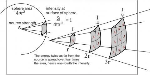
Any point source which spreads its influence equally in all directions without a limit to its range will obey the inverse square law. This phenomenon is based on strictly geometrical considerations. In Figure A.1, the intensity I of the influence at any given radius r is equal to the source strength S divided by the area (4πr2) of the sphere.
Figure A.1. Logical view of the "Inverse-Square-Law" (Courtesy of HyperPhysics)
A.2 Air Kerma
Air kerma is the radiation concentration delivered to a point at a certain distance away from the source.
The quantity, kerma, originated from the acronym, KERMA (Kinetic Energy Released per unit MAss). It is a measure of the amount of radiation energy, in the unit of joules (J), actually deposited in, or absorbed, in a unit mass (kg) of air. Therefore, the quantity, kerma, is expressed in the units of J/kg which is also the radiation unit, the gray (Gy).
Following the definition, the measurement of the activity A at the distance d from the source, the Air Kerma is expressed as follows:
$K=\frac{A \cdot \gamma \cdot 10^6}{d^2}$ (A.1)
where, γ is a constant of a particular radio-isotope, which is measured in Gy·m2/s·Bq. It can be noticed that Eq. (1) holds the intrinsic property of the inverse square-law.
The activity A of the sample used by us to define the Air kerma represents the number of disintegrations taking place per time unit. The activity also represents the number of gamma rays emitted.
A.3 Equivalent dose
Equivalent dose e is the quantity commonly used to express the biological impact of radiation. This entity must be calculated first in order to calculate the total effective dose.
e=K·q (A.2)
Equivalent dose is proportional to the air kerma and the quality factor q that is dependent on the radio isotope.
A.4 Effective dose
Effective dose is a very useful radiation quantity for expressing relative risk to humans. This quantity is indeed the expressed quantity by most of the commercial radiation detectors such as a GM counter. For the purpose of determining the effective dose, the different areas and organs have been assigned tissue weighting factor values. If more than one area has been exposed, then the total body tissue weighting factor Q is just the sum of the tissue weighting factors for each exposed organ, where Q=1 represents the standard value.
Effective dose is expressed as follows:
E=e·Q (A.3)
The UM of effective (equivalent) dose is Sv/s. Since the GM counter acquires the dose in µSv/h, for our calculation convenience we have converted Sv/s into µSv/h as:
$E=\frac{3.6 \cdot 10^{15} \cdot A \cdot \gamma \cdot q \cdot Q}{d^2}$ (A.4)
where, the equivalent dose e was replaced with Eq. (1) and (2).
A.5 Quality factor
The quality factor, q is a dimension less modifier used in converting absorbed dose, expressed in rads (or grays), to dose equivalent, expressed in rems (or sieverts). The dose equivalent is used in radiation protection to account for the biological effectiveness of different kinds of radiation. The quality factor is related to both the linear energy transfer and relative biological effectiveness.
[1] Bristow, Q. (1978). The application of airborne gamma-ray spectrometry in the search for radioactive debris from the Russian satellite COSMOS 954 (Operation ‘Morning Light’). Geological Survey of Canada, 78: 151-162.
[2] Che, J., Wang, J., Li, K. (2014). A Monte Carlo based robustness optimization method in new product design process: A case study. American Journal of Industrial and Business Management, 4(7): 10. https://doi.org/10.4236/ajibm.2014.47044
[3] Wang, X., Yan, L., Zhang, Q. (2021). Research on the application of gradient descent algorithm in machine learning. In 2021 International Conference on Computer Network, Electronic and Automation (ICCNEA), pp. 11-15. https://doi.org/10.1109/ICCNEA53019.2021.00014
[4] INCLUDING project. European Commission (H2020/2013-2020). https://including-cluster.eu/
[5] Molnar, A., Domozi, Z., Lovas, I. (2021). Drone-based gamma radiation dose distribution survey with a discrete measurement point procedure. Sensors, 21(14): 4930. https://doi.org/10.3390/s21144930
[6] Christie, G., Shoemaker, A., Kochersberger, K., Tokekar, P., McLean, L., Leonessa, A. (2017). Radiation search operations using scene understanding with autonomous UAV and UGV. Journal of Field Robotics, 34(8): 1450-1468. https://doi.org/10.1002/rob.21723
[7] Li, B., Zhu, Y., Wang, Z., Li, C., Peng, Z.R., Ge, L. (2018). Use of multi-rotor unmanned aerial vehicles for radioactive source search. Remote Sensing, 10(5): 728. https://doi.org/10.3390/rs10050728
[8] Steinhäusler Friedrich, Zaitseva Lyudmila, Kolovos Spyros, Nadzieko Aleksandra, De Dominicis Luigi, Heikkinen Isto, & Jyri Silmari. (2022). The G516 gap: Lack of small (capable of low flying) UAVs with payload high enough to carry out radiation measurements. Zenodo. https://doi.org/10.5281/zenodo.6349422
[9] Sanada, Y., Torii, T. (2015). Aerial radiation monitoring around the Fukushima Dai-ichi nuclear power plant using an unmanned helicopter. Journal of Environmental Radioactivity, 139: 294-299. https://doi.org/10.1016/j.jenvrad.2014.06.027
[10] Bristow, Q. (1978). The application of airborne gamma-ray spectrometry in the search for radioactive debris from the Russian satellite COSMOS 954 (Operation ‘Morning Light’). Geological Survey of Canada, 78: 151-162.
[11] Gandhi, S.S. (1978). Geological observations and exploration guides to uranium in the Bear and Slave structural provinces and the Nonacho Basin, District of Mackenzie. Current Research, Part B, Geol. Surv. Can., Paper 78-1B, p. 141-149.
[12] IAEA Action Plan on Nuclear Safety, IAEA, 2011.
[13] Torabbeigi, M., Lim, G.J., Kim, S.J. (2020). Drone delivery scheduling optimization considering payload-induced battery consumption rates. Journal of Intelligent & Robotic Systems, 97: 471-487. https://doi.org/10.1007/s10846-019-01034-w