Suha S. Husain* | Taghreed MohammadRidha
© 2022 IIETA. This article is published by IIETA and is licensed under the CC BY 4.0 license (http://creativecommons.org/licenses/by/4.0/).
OPEN ACCESS
Reducing the seismic effect is important to ensure people's safety and structures to remain operational even after the earthquakes. Therefore, many studies have been carried out in this filed in recent years. In this study three types of sliding mode control are designed to reduce the effect of vibration on buildings during an earthquake. An Active Tuned Mass Damper (ATMD) is used in this study as an actuator to absorb seismic vibration. Classical Sliding Mode Control (SMC), Integral Sliding Mode Control (ISMC) and Integral Sliding Mode Control based on barrier function (ISMCbf) are designed to control the performance of ATMD to reduce structural vibrations under effect of earthquake excitation. The three types of controllers are compared under effect of two types of earthquakes: El Centro 1940 earthquake and Mexico City earthquake. This comparison shows that ISMCbf has many advantages, firstly, it does not require prior knowledge of the bounds of disturbances and uncertainties. Secondly, ISMCbf is chattering free, thus, it does need any type of approximation to avoid chattering phenomenon. Finally, the numerical simulation results showed that the state trajectory is confined within the barrier of the sliding manifold and provided a better performance.
sliding mode control, integral sliding mode control, ATMD, active control, seismic effect control, structural vibration, earthquakes
One of the main goals of civil engineering is to design safe and comfortable buildings to their users. To achieve this goal, buildings should maintain stability by resisting external disturbances such as wind and earthquakes. The increase in population led to the necessity of constructing multi-story buildings. Conventional seismic structural design attempts to construct buildings that do not collapse under strong earthquake excitations, but damage of non-structural elements may not be avoided. This can render the building non-functional after the earthquake, which may be problematic in some structures, like hospitals, which need to remain functional after earthquake.
Two basic technologies are used to protect buildings from damaging earthquake effects. These are base isolation devices (passive control) and seismic dampers (active, hybrid and semi-active control) [1]. The idea behind base isolation is to detach (isolate) the building from the ground in such a way that earthquake motions are not transmitted up through the building, or at least greatly reduced. Isolation techniques are good choice but not sufficient in some cases and they are passive devices (uncontrolled) [2].
On the other hand, there are active control devices that work in the presence of external forces generated by actuators such as Active Tuned Mass Damper (ATMD). These are transmitted through the structure and give a response that reduces the seismic effects [3]. Active control devices are areal time control [4]. The combination of the two previous types produces the so called hybrid control system. Its active portion is only used when there is high building excitation, otherwise, it behaves passively. The force of these devices is adjustable based on the control of fluid viscosity using electrical or magnetic fields supplied by low-power batteries such as a magneto rheological fluid damper (MRD) [5].
Many researchers have been involved in this field, some of them adopted classical control methods like [6] where the authors suggested MRD to control a three story scaled structure with Linear Quadratic Regulator (LQR) controller, El Ouni et al. [7] studied the effect of adding shear walls with active control. Others relied on robust control. In previous two studies the authors proposed classical controllers which are not sufficient to control the systems with perturbations.
Moreover, Wasilewski et al. [8] designed an active control system for 20-story large scale structure and compared three types of controllers: Linear-quadratic-Gaussian (LQG) regulator, H∞ and adaptive optimal control. These types of controllers were checked under different earthquake simulations (Kobe earthquake, El Centro earthquake, Sine signal and Poly harmonic signal). The acceleration drift was minimized to 50% using adaptive control as compared to the other controllers.
Fali et al. [9] and Humaidi et al. [10] proposed adaptive sliding mode control (ASMC) to control a three story scaled structure then compared it with classical SMC. They used MRD as an actuator. They concluded that the adaptive gain of ASMC varies between the upper and lower bounds of sliding gain depending on the perturbations bounds. Khatibinia et al. [11] designed Optimal Sliding Mode Control (OSMC) to control a 11-story building with ATMD installed on the top floor. They compared OSMC with PID controller, LQR and fuzzy logic controller (FLC) under simulated earthquakes. They concluded that OSMC can further reduce the displacement by 36.7%. Concha et al. [12] proposed an automatic tuning algorithm to design SMC to control an ATMD to reduce vibration effect on structures. They compared SMC with LQR and concluded that SMC performance dominated the LQR results.
As presented above, SMC is proved to be one of the reliable robust controllers for such systems under severe external disturbances. However, from the previous studies it is noticed that SMC, ASMC and OSMC need the perturbations upper bounds in the design procedure. Moreover, these robust controllers usually need kind of approximation to avoid chattering phenomenon caused by discontinuous term in controller design.
In this work, Integral Sliding Mode Control Based on Barrier Function (ISMCbf) is designed for the first time for this application. It is chosen due to its robustness and design simplicity where the upper bound of external disturbances is not required in the design procedure [13]. Moreover, ISMCbf does not have a discontinues term hence, it is a chattering-free SMC type as will be shown later. ISMCbf is designed to control ATMD that is placed on the top floor of a 5-story scaled building exposed to El Centro earthquake. The results are compared to SMC performance [12]. Simulation results show that ISMCbf is efficient in reducing structural displacement and control effort as well. Moreover, the proposed control algorithm is more robust and simpler in design as compared to other SMC types.
This paper organized as follows: the mathematical model of a building with ATMD section 2. Sliding mode control design explained in section 3. Thereby, in section 4 the results were presented and discussed. Finally, this study was concluded with the conclusion section 5.
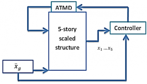
Figure 1. A building with ATMD on the top floor
A 5-story scaled structure is employed in this work in Figure 1. This scaled model is described by the following differential equations [12]:
$M \ddot{\boldsymbol{x}}(t)+C \dot{\boldsymbol{x}}(t)+K \boldsymbol{x}(t)=-M I \ddot{x}_g(t)-\Gamma F(t)$ (1)
$m_d \ddot{x}_d(t)+m_d \ddot{x}_n(t)+m_d \ddot{x}_g(t)=F(t)$ (2)
$F(t)=u(t)-k_d x_d(t)-c_d \dot{x}_d(t)-f\left(\dot{x}_d(t)\right)$ (3)
where, $C, K$ and $M \in R^{n * n}$ are damping, stiffness and mass matrices. $M$ is a diagonal matrix. $C$ and $K$ are tridiagonal matrices. $\ddot{x}_g$ is the earthquake acceleration, the vector $\boldsymbol{x}=$ $\left[x_1, x_2, x_3, \ldots, x_n\right]^T$ where $x_i$ represents the displacement of the ith floor related to the ground floor and $n=5$. $x_d, m_d, c_d, k_d$ and $f\left(\dot{x}_d\right)$ are the displacement, mass, damping, stiffness and non-linear friction of the ATMD, respectively. $F$ is the force acting upon the ATMD. $u(t)$ is the control force applied to ATMD, $I \epsilon R^{n * n}$ is unity vector, $\Gamma \in R^{n * n}$ represent the location of ATMD as the follows:
$\Gamma=[0,0,0, \ldots, 1]^T$
The structural dominant mode during an earthquake is the first mode of the building with ATMD, which represents approximately the building for control purposes. It can be approximated as [12]:
$m_0 \ddot{x_0}(t)+c_0 \dot{x_0}(t)+k_0 x_0(t)$$=-b_0 m_0 \ddot{x}_g(t)-F(t)$ (4)
$m d\left(\ddot{x_0}(t)+\ddot{x d}(t)+\ddot{x_g}(t)\right)=F(t)$ (5)
where, $x_0, m_0, c_0$ and $k_0$ are the displacement, mass, damping and stiffness of the dominant mode respectively, which are given by [12]:
$x_0(t)=\frac{\phi^T M \boldsymbol{x}(t)}{\phi^T M \phi}$ (6)
$m_0=\phi^T M \phi$ (7)
$c_0=\phi^T C \phi$ (8)
$k_0=\phi^T \mathrm{~K} \phi$ (9)
$M b_0=\frac{\phi^T M I}{\phi^T M \phi}$ (10)
where, $\Phi \in R^{n * n}$ that satisfy:
$\phi^T \Gamma=1$ (11)
This equality led to this approximation:
$x_n(t) \approx x_0(t)$ (12)
The dominant mode natural frequency is given by [12]:
$\omega=\sqrt{\frac{k_0}{m_0}}$ (13)
Using the approximation in Eq. (12) then substituting $F(t)$ in Eq. (3) in to Eq. (4) and (5) [12]:
$\ddot{x}_n=-\frac{c_0}{m_0} \dot{x}_n-\frac{k_0}{m_0} x_n-b_0 \ddot{x}_g+\frac{c_d}{m_0} \dot{x}_d+\frac{k d}{m_0} x d$$+\frac{f(\dot{x} d)}{m_0}-\frac{1}{m_0} u$ (14)
$\ddot{x}_d=\left(\frac{m_0+m d}{m_0 m d}\right)\left(u-c_d \dot{x} d-f\left(\dot{x}_d\right)-k_d x_d\right)$$+\frac{k_0}{m_0} x_n+\frac{c_0}{m_0} \dot{x}_n+\left(b_0-1\right) \ddot{x}_g$ (15)
The state variables are defined as the follows:
$z_1=x_d \quad z_2=x_n \quad z_3=\dot{x}_d \quad z_4=\dot{x}_n$ (16)
Rewriting the system in Eqns. (14) and (15) using the new state variables in Eq. (16) as [12]:
$\dot{\boldsymbol{z}}=A \boldsymbol{z}+B\left(u-f\left(z_3\right)\right)+D \ddot{x}_g$ (17)
where: $A=\left[\begin{array}{cccc}0 & 0 & 1 & 0 \\ 0 & 0 & 0 & 1 \\ -\frac{k d\left(m_0+m d\right)}{m_0 m d} & \frac{k_0}{m_0} & -\frac{c d\left(m_0+m d\right)}{m_0 m d} & \frac{c_0}{m_0} \\ \frac{k d}{m_0} & \frac{-k_0}{m_0} & \frac{c d}{m_0} & \frac{-c_0}{m_0}\end{array}\right]$, $\mathbf{z}=\left[\begin{array}{l}z_1 \\ z_2 \\ z_3 \\ z_4\end{array}\right], \quad B=\left[\begin{array}{c}0 \\ 0 \\ \frac{\left(m_0+m d\right)}{m_0 m d} \\ \frac{-1}{M 0}\end{array}\right], \quad D=\left[\begin{array}{c}0 \\ 0 \\ b_0-1 \\ -b_0\end{array}\right]$.
$f\left(z_3\right)=\mu_d \operatorname{sgn}\left(z_3\right)$
The above dominant mode model will be used for the control design purposes.
Sliding mode control is a robust controller that has two phases, reaching phase and sliding phase [14, 15]. It can reject the effect of matched disturbances and uncertainties during the sliding phase. The sliding manifold is designed to be attractive and invariant. Therefore, SMC is a good choice for systems where the controller and the disturbance are in the same channel [16].
ISMC has no reaching phase and sliding occurs from the first instance. Hence, the system is not affected by the undesired external inputs as it is imposed to remain on the sliding manifold. Moreover, ISMC can guarantee that unmatched disturbances are not amplified via a good selection of sliding surface [17, 18]. For both classical SMC and ISMC, the bounds of the matched disturbances and uncertainties are needed. A new ISMCbf [19] is designed here which does not require the prior knowledge of the bounds of disturbances and uncertainties. Only one parameter is to be chosen, as will be shown in subsection 3.3.
Classical SMC, ISMC and ISMCbf are designed next to compare their performances.
3.1 Classical ISMC design
Classical ISMC is designed for the dominant mode model in Eq. (17). First define the switching variable [17]:
$\sigma=G \boldsymbol{z}+Y$ (18)
The vector $G$ is given by:
$G=\left[\begin{array}{llll}g_1 & g_2 & g_3 & g_4\end{array}\right]$ (19)
where, $g_1, \ldots g_4$ are design parameters. $Y$ is the integral term whose dynamics is described in Eq. (20) [17];
$\dot{Y}=-G A z-u_n$ (20)
ISMC control law is as follows:
$u_{=}(G B)^{-1}\left(u_n+u_s\right)$ (21)
$u_s=-K_0 \operatorname{sign}(S)$ (22)
$u_n=-K \boldsymbol{z}$ (23)
where, $u_n$ is a nominal controller which provides the nominal system performance, $u_s$ is the discontinuous control which handles disturbances and uncertainties [20]. $K_0$ is a positive switching gain that will be designed depending on the upper bound of the perturbation. In this way the discontinuous control term $u_s$ will compensate the perturbation effect. $K$ is a gain vector which can be designed by using Ackermann's formula. $G$ is designed such that $(G B)$ is invertible.
To ensure the attractiveness of the sliding manifold $\sigma$ the condition in Eq. (24) must be satisfied [21]:
$\sigma \dot{\sigma}<0$ (24)
The dynamics of the sliding manifold $\sigma$ which used in Eq. (24) is:
$\dot{\sigma}=G \dot{\boldsymbol{z}}+\dot{Y}=G\left(A \boldsymbol{z}+B\left(u-f\left(z_3\right)\right)+D \ddot{x}_g\right)+\dot{Y}$ (25)
The condition (24) becomes:
$\sigma \dot{\sigma}=\left(\sigma G\left(A Z+B\left(u-f\left(z_3\right)\right)+D \ddot{x}_g\right)+\dot{Y}\right)<0$ (26)
Assumption 1. The earthquake acceleration $\ddot{x} g$ and the non-linear friction $f\left(z_3\right)$ are assumed to be unknown but bounded by known positive quantities $\delta$ and $\tilde{\omega}$ respectively [12]:
$|\ddot{x} g| \leq \delta$ (27)
$\left|f\left(z_3\right)\right| \leq \tilde{\omega}$ (28)
Using Eqns. (21), (22) and (23), and taking the above upper bounds into consideration in Eq. (26), the result is;
$\sigma \dot{\sigma} \leq-|\sigma|\left(K_0+G B \tilde{\omega}-G D \delta\right)$ (29)
$K_0$ is designed to ensure attractiveness condition (24) i.e.:
$K_0>G D \delta-G B \tilde{\omega}$ (30)
During sliding $\sigma=0, \dot{\sigma}=0$, the equivalent of the discontinuous control is yielded $\left[u_s\right]_{e q}$
$\left[u_s\right]_{e q}=G B \tilde{\omega}-G D \delta$ (31)
Thus, the equivalent system dynamics during the sliding phase becomes:
$\dot{\boldsymbol{z}}=(A-B K) \boldsymbol{z}$ (32)
Finally, ISMC is as follows:
$u=(G B)^{-1}\left(-G A \boldsymbol{z}-K \boldsymbol{z}-K_0 \operatorname{sign}(\sigma)\right)$ (33)
3.2 Integral sliding mode based on barrier function
In this study ISMCbf is used as it does not require the perturbations bounds and it is inherently continuous. The design principle is based on replacing the discontinuous control term $u_c$ by a barrier function. The barrier function provides a simpler ISMC design as it does not require any information regarding the bounds of the unknown disturbance as classical SMC and ISMC do [19, 22]. Moreover, it provides a continuous control without the high frequency chattering that is present in the classical SMC and ISMC as shown in Eq. (33).
Two types of barrier function exist: Positive definite BFs (PBFs) and Positive Semi-definite BFs (PSBFs) [19, 22]. PSBFs is used in this work. ISMCbf design procedure does not differ from ISMC design presented earlier, only the discontinuous term is replaced as follows [22]:
$\sigma=G \boldsymbol{z}+Y$ (34)
$\dot{Y}=-G A \boldsymbol{z}-u_n$ (35)
$u_n=-K \boldsymbol{z}$ (36)
$u_s=-\frac{\sigma}{\epsilon-|\sigma|}$ (37)
$u=(G B)^{-1}\left(u_n+u_s\right)$ (38)
where, $\epsilon$ is very small positive number. Finally, ISMCbf is as follows:
The attractiveness of the sliding manifold is verified by:
$\sigma \dot{\sigma}=\sigma\left(-\frac{\sigma}{\epsilon-|\sigma|}-G B f\left(z_3\right)+G D \ddot{x}_g\right)<0$ (39)
Let $-G B f\left(z_3\right)+G D \ddot{x}_g=\delta_1$
$\sigma \dot{\sigma} \leq-|\sigma|\left(\frac{|\sigma|}{|\epsilon-| \sigma||}-\left|\delta_1\right|\right)$ (40)
So $\sigma \dot{\sigma}<0$ for $|\sigma|$ sufficiently near $\epsilon$ where $\frac{|\sigma|}{|\epsilon-| \sigma||}>\left|\delta_1\right|$.
As shown, the main advantage of ISMCbf is that the upper bound of parameters uncertainty and disturbances are not required [19, 21]. Only one control parameter is to be chosen that is $\epsilon$, which is very small positive constant.
To compare the performance of the proposed control algorithm, classical SMC will also be designed in the following subsection.
3.3 Classical SMC design
The design procedure of SMC which used in the study of Concha et al. [12] will be followed in this work. The sliding manifold is defined as [12]:
$\sigma=G \boldsymbol{Z}$ (41)
SMC control action is as follows:
$u=-K_0 \operatorname{sign}(\sigma)$ (42)
The switching gain $K_0$ is choose to insure the attractiveness of sliding manifold [12]:
$K_0>\tilde{\omega}+h_0$ (43)
where, $h_0$ is defined as follows [12]:
$h_0=\left|-K z+\alpha_1 \ddot{x}_g\right|$ (44)
$\alpha_1=b_0\left(g_4-g_3\right)+g_3$ (45)
For more details see the study of Concha et al. [12].
This section presents the simulation results of 5-story scaled structure with three types of sliding mode controllers to drive the ATMD. All results are obtained by Matlab/ Simulink environment. The initial condition of Eq. (17) is set to zero $(\boldsymbol{x}(0)=0)$; the gain vector $K$ is designed by Ackermann's formula according to the desired characteristic Eq. (46). It is chosen based on the selection of the desired damping ratio and the natural frequency $\zeta$ and $w_n$ respectively [12]:
$\left(s^2+2 \zeta \omega_n+\omega_n^2\right)\left(s+\lambda_3\right)\left(s+\lambda_4\right)$ (46)
$\lambda_{1,2}=-\zeta \omega_n \pm j \omega_d, \lambda_3=-3 \zeta \omega_n$ (47)
$\lambda_4$ is any negative value. Where $w_d$ is the damped natural frequency expressed as $\lceil 12\rceil$ :
$\omega_d=\omega_n \sqrt{1-\zeta^2}$ (48)
$w_n$ is chosen based on frequency of the dominant mode $w_0$. The feasible range of $w_n$ is [12]:
$\omega_{n l}<\omega_n<\omega_{n u}$ (49)
where, $\omega_{n l}=0.5 \omega_0$ and $\omega_{n u}=0.8 \omega_0$. Note that if $w_n$ is selected near $w_0$ then a sudden movement may occur, on the other hand if $w_n$ is selected $0.5 w_0$ the transient response will be very slow. $\zeta$ is within [12]:
$\zeta_l$<$\zeta$<$\zeta_u$ (50)
where, $\zeta_l=0.5, \zeta_u=0.9$.
The desired $\zeta, \omega_n$ and $\omega_0$ are given in Table 1 . It is good to mention that these values of $(\zeta)$ and $\left(w_n\right)$ provide a better damping behaviour than the values given in [12].
A well-known fact of $\mathrm{SMC}$ is that the discontinues term $u_s$ in SMC and ISMC cause chattering phenomenon, where chattering is a finite amplitude signal with high frequency [23, 24]. Hence, to avoid chattering, the following approximation is used in Eqns. (33) and (42) [12]:
$\operatorname{sign}(\sigma) \approx \frac{\sigma}{|\sigma|+\alpha}$ (51)
where, $\alpha$ is very small positive value given in Table 2.
Table 1. Design parameters of model and ATMD [12]
|
Parameter |
Value |
|
$m_0, k_0, b_0$ |
28.07 kg, 2.75 ×10 N/m, 1 |
|
$c_0$ |
Calculated by Rayleigh damping, with damping ratios 0.01 |
|
$m_d, c_d k_d$ |
1.4 kg, 3.54 Ns/m, 121.66 N/m, |
|
$\mu_d, w_0$ |
0.35 N, 9.9 rad/s |
Table 2. Control parameters
|
Parameter |
Value |
|
$G$ |
$\left[\begin{array}{llll}0 & 0 & 0 & 1\end{array}\right]$ |
|
$\zeta, w_n$ |
$0.7,0.8 w_0$ |
|
$\lambda_{1,2}, \lambda_3, \lambda_4$ |
$-5.44 \pm j 2.24,-16.632,-28$ |
|
$\epsilon, \alpha$ |
0.005, 0.005 |
As mentioned earlier ISMCbf does not require a prior knowledge of the perturbation upper bounds. Therefore, to prove this the design is tested under two different earthquakes with the same ISMCbf design. The simulation results presented below compares three types of controllers (SMC, ISMC and ISMCbf) under effect of time scaled El Centro 1940 earthquake. To show the robustness of the proposed controller, all three controllers are compered under a different disturbance which is the time scaled Mexico City earthquake. The open-loop uncontrolled top floor displacement under El Centro 1940 time scale earthquake is illustrated in Figure 2 and 3 respectively.
Figure 2. Uncontrolled top floor displacement effected by El Centro 1940 time scale earthquake
Figure 3. El Centro 1940 time scale earthquake
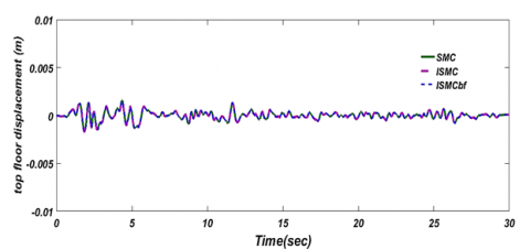
Figure 4. Displacement of the top floor with SMC, ISMC and ISMCbf
SMC, ISMC and ISMCbf control actions in Eqns. (24), (36) and (47) are applied respectively to control the system. Figure 4 shows the result of top floor displacement with SMC, ISMC and ISMCbf.
Control action of SMC, ISMC and ISMCbf are shown in Figure 5.
Figure 5. Control action with SMC, ISMC and ISMCbf
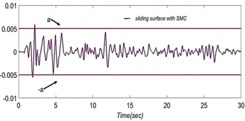
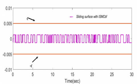
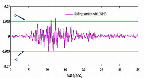
Sliding surfaces of SMC, ISMC and ISMCbf in Eqns. (18), (34) and (41) are shown in Figure 6. Notice that the sliding variable of ISMCbf is confined in the invariant set $\sigma<|\epsilon|$.
(a)
(b)
(c)
Figure 6. The sliding surface of SMC, ISMC, ISMCbf respectively
Table 3. Maximum structural displacement and control action under El Centro1940 earthquake
|
|
Open-loop |
SMC |
ISMS |
ISMCbf |
|
Maximum first floor displacement (m) |
0.0024 |
0.0008 |
0.0008 |
0.0008 |
|
Maximum second floor displacement (m) |
0.004 |
0.0013 |
0.0013 |
0.0013 |
|
Maximum third floor displacement (m) |
0.0055 |
0.0016 |
0.0016 |
0.0016 |
|
Maximum fourth floor displacement (m) |
0.008 |
0.00178 |
0.00178 |
0.00178 |
|
Maximum top floor displacement (m) |
0.01 |
0.002 |
0.002 |
0.002 |
|
Maximum control action (N) |
- |
15 |
10.64 |
10.64 |
The statistical results of the compared controllers under effect of time scaled El Centro 1940 earthquake are given in Table 3. From these results it is clear that both SMC, ISMC and ISMCbf succeeded in reducing structural displacement in the same rate but with deferent control force, ISMC and ISMCbf reduced the control force by (33%) as compared to SMC.
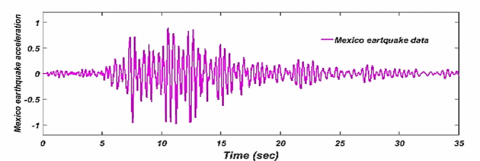
A second case study is taken here where the system is exposed to the time scaled Mexico City earthquake which is shown in Figure 7. The purpose of this test is to show the robustness of ISMCbf under different disturbances without the need of any information of the perturbations bounds in the both cases.
Figure 7. Time scaled Mexico City earthquake
Figure 8. Uncontrolled top floor displacement effected by time scaled Mexico City earthquake
Figure 9. The displacement of the top floor controlled by SMC, ISMC and ISMCbf respectively
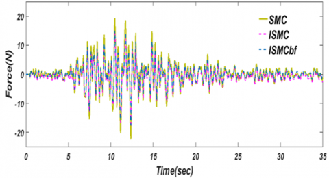
Figure 10. Control action with SMC, ISMC and ISMCbf
The uncontrolled building displacement under time scaled Mexico City earthquake is shown in Figure 8.
Controlled top floor displacement and controlled force of SMC, ISMC and ISMCbf are shown in Figures 9 and 10 respectively.
Sliding surfaces for SMC, ISMC and ISMCbf are shown in Figure 11.
(a)
(b)
(c)
Figure 11. The sliding surface of SMC, ISMC, ISMCbf respectively
Table 4. Maximum structural responses under the Mexico City earthquake
|
|
Open-loop |
SMC |
ISMS |
ISMCbf |
|
Maximum first floor displacement (m) |
0.0055 |
0.0028 |
0.0028 |
0.0028 |
|
Maximum second floor displacement (m) |
0.01 |
0.00365 |
0.00365 |
0.00365 |
|
Maximum third floor displacement (m) |
0.0135 |
0.0048 |
0.0048 |
0.0048 |
|
Maximum fourth floor displacement (m) |
0.0185 |
0.0057 |
0.0057 |
0.0057 |
|
Maximum top floor displacement (m) |
0.022 |
0.0065 |
0.0065 |
0.0065 |
|
Maximum control action (N) |
- |
19.5 |
15 |
15 |
The statistical results of effect of Mexico City earthquake case study are presented in Table 4. The same conclusion of the first case study is yielded here, in terms of the applied and required control energy there is significant differences as shown in Table 4. ISMC and ISMCbf reduced control action about (33%) as compared to SMC to get the same displacement reduction.
From the results, it is clear that ISMCbf deals with two different bounds of disturbances without needing to update the design parameters (no change of control design).
In this study ISMCbf is designed for the first time to reduce structural displacement due to seismic effect with ATMD. The main advantage which distinguishes ISMCbf from ISMC and SMC is that ISMCbf does not need any information about the upper bounds of the disturbances in the design. Only one parameter is to be specified which represents a small positive constant. The simulation results in the presence of earthquake show that ISMCbf and ISMC has the minimum control action as compared to SMC with the same disturbance rejection performance. Moreover, to reduce chattering in ISMC and SMC, a sigmoid function is utilized which adds another design parameter to be specified. ISMCbf prevents chattering as it is a continuous controller therefore, there is no need for this kind of approximation. Hence, ISMCbf proved to be more efficient and simpler in the design.
ISMCbf proves its efficiency with ATMD, but ATMD has some disadvantages, like high power requirements and thus a high cost. Moreover, ATMD performance has a constraint in its design and implementation. Therefore, as a future work, it is suggested to replace ATMD with MRD which is known to be more reliable, have a low power requirement and of low cost and easy to install and maintain.
[1] Chang, C.M., Shia, S., Lai, Y.A. (2018). Seismic design of passive tuned mass damper parameters using active control algorithm. Journal of Sound and Vibration, 426: 150-165. https://doi.org/10.1016/j.jsv.2018.04.017
[2] Cancellara, D., Pasquino, M. (2011). A new passive seismic control device for protection of structures under anomalous seismic events. In Applied Mechanics and Materials, 82: 651-656. https://doi.org/10.4028/www.scientific.net/AMM.82.651
[3] Ulusoy, S., Nigdeli, S.M., Bekdaş, G. (2021). Novel metaheuristic-based tuning of PID controllers for seismic structures and verification of robustness. Journal of Building Engineering, 33: 101647. https://doi.org/10.1016/j.jobe.2020.101647
[4] Saidi, A., Zizouni, K., Kadri, B., Fali, L., Bousserhane, I.K. (2019). Adaptive sliding mode control for semi-active structural vibration control. Studies in Informatics and Control, 28(4): 371-380. https://sic.ici.ro/wp-content/uploads/2019/12/Art.-1-Issue-4-SIC-2019.pdf.
[5] Fu, W., Zhang, C., Li, M., Duan, C. (2019). Experimental investigation on semi-active control of base isolation system using magnetorheological dampers for concrete frame structure. Applied Sciences, 9(18): 3866. https://doi.org/10.3390/app9183866
[6] Zizouni, K., Bousserhane, I.K., Hamouine, A., Fali, L. (2017). MR Damper-LQR control for earthquake vibration mitigation. International Journal of Civil Engineering and Technology (IJCIET), 8(11): 201-207.
[7] El Ouni, M.H., Laissy, M.Y., Ismaeil, M., Ben Kahla, N. (2018). Effect of shear walls on the active vibration control of buildings. Buildings, 8(11): 164. https://doi.org/10.3390/buildings8110164
[8] Wasilewski, M., Pisarski, D., Bajer, C.I. (2019). Adaptive optimal control for seismically excited structures. Automation in Construction, 106: 102885. https://doi.org/10.1016/j.autcon.2019.102885
[9] Fali, L., Djermane, M., Zizouni, K., Sadek, Y. (2019). Adaptive sliding mode vibrations control for civil engineering earthquake excited structures. International Journal of Dynamics and Control, 7(3): 955-965. https://doi.org/10.1007/s40435-019-00559-0
[10] Humaidi, A.J., Sadiq, M.E., Abdulkareem, A.I., Ibraheem, I.K., Azar, A.T. (2022). Adaptive backstepping sliding mode control design for vibration suppression of earth-quaked building supported by magneto-rheological damper. Journal of Low Frequency Noise, Vibration and Active Control, 41(2): 768-783. https://doi.org/10.1177/1461348421106465
[11] Khatibinia, M., Mahmoudi, M., Eliasi, H. (2020). Optimal sliding mode control for seismic control of buildings equipped with ATMD. Iran University of Science & Technology, 10(1): 1-15. http://ijoce.iust.ac.ir/article-1-417-en.html.
[12] Concha, A., Thenozhi, S., Betancourt, R.J., Gadi, S.K. (2021). A tuning algorithm for a sliding mode controller of buildings with ATMD. Mechanical Systems and Signal Processing, 154: 107539. https://doi.org/10.1016/j.ymssp.2020.107539
[13] Obeid, H., Fridman, L.M., Laghrouche, S., Harmouche, M. (2018). Barrier function-based adaptive sliding mode control. Automatica, 93: 540-544. https://doi.org/10.1016/j.automatica.2018.03.078
[14] Humaidi, A.J., Hasan, S., Al-Jodah, A.A. (2018). Design of second order sliding mode for glucose regulation systems with disturbance. International Journal of Engineering & Technology, 7(2.28): 243-7.
[15] Ridha, T.M.M. (2010). The design of a tuned mass damper as a vibration absorber. Engineering and Technology Journal, 28(14): 4844-4852.
[16] Mahmoud, U.Y., Yasien, F.R., Ridha, T.M.M. (2009). Sliding mode control for gust responses in tall building. Engineering and Technology Journal, 27(5): 982-992.
[17] Hamayun, M.T., Edwards, C., Alwi, H. (2016). Fault Tolerant Control Schemes Using Integral Sliding Modes. Switzerland: Springer International Publishing.
[18] De Loza, A.F., Bejarano, F.J., Fridman, L. (2013). Unmatched uncertainties compensation based on high‐order sliding mode observation. International Journal of Robust and Nonlinear Control, 23(7): 754-764. https://doi.org/10.1002/rnc.2795
[19] Obeid, H., Fridman, L., Laghrouche, S., Harmouche, M. (2018). Barrier function-based adaptive integral sliding mode control. In 2018 IEEE Conference on Decision and Control (CDC), pp. 5946-5950. https://doi.org/10.1109/CDC.2018.8619334
[20] Pan, Y., Yang, C., Pan, L., Yu, H. (2017). Integral sliding mode control: Performance, modification, and improvement. IEEE Transactions on Industrial Informatics, 14(7): 3087-3096. https://doi.org/10.1109/TII.2017.2761389
[21] Ezzaldean, M.M., Kadhem, Q.S. (2019). Design of control system for 4-switch BLDC motor based on sliding-mode and hysteresis controllers. Iraqi Journal of Computers, Communications, Control and Systems Engineering, 19(1): 42-51. https://doi.org/10.33103/uot.ijccce.19.1.6
[22] Abd, A.F., Al-Samarraie, S.A. (2021). Integral sliding mode control based on barrier function for servo actuator with friction. Engineering and Technology Journal, 39(2): 248-259. https://doi.org/10.30684/etj.v39i2A.1826
[23] Bartolini, G., Ferrara, A., Usai, E. (1998). Chattering avoidance by second-order sliding mode control. IEEE transactions on Automatic Control, 43(2): 241-246. https://doi.org/10.1109/9.661074
[24] Rakan, A.B., MohammadRidha, T., AL-Samarraie, S.A. (2022). Artificial pancreas: Avoiding hyperglycemia and hypoglycemia for type one diabetes. International Journal on Advanced Science, Engineering and Information Technology, 12(1): 194-201. https://doi.org/10.18517/ijaseit.12.1.15106