Maurizio Carbone* | Michele Iovieno
© 2020 IIETA. This article is published by IIETA and is licensed under the CC BY 4.0 license (http://creativecommons.org/licenses/by/4.0/).
OPEN ACCESS
The ability of the non-uniform Fast Fourier Transform (NUFFT) to predict the particle feedback on the flow in particle-laden flows in the two-way coupling regime is examined. In this regime, the particle back-reaction on the fluid phase can substantially modify the flow statistics across all the scales, when particle loading is significant. While many works in the literature focus on the direct B-spline interpolation, which is now a well-established method for the one-way coupling, only a few methods are available for the computation of particle back-reaction, which are often lower order and reduce the overall accuracy of the simulation. In our implementation, particle momentum and temperature back-reactions on the fluid flow are computed by means of the forward NUFFT with B-spline basis, while the B-spline interpolation is performed as a backward NUFFT. An application of the NUFFT to the simulation of a statistically steady and isotropic turbulent flow, laden with inertial particles is presented. The effect of particle feedback on velocity and temperature structure functions and on particle clustering is discussed as a function of the Stokes number, together with the spectral characterization of the particle phase.
direct numerical simulation, particle-laden flows, two-way coupling, turbulence
The transport of particles suspended in a turbulent flow plays a central role in many physical and engineering problems, from combustion engines to the cooling of miniaturized components [1, 2], from cloud microphysics to sediment distribution in aquatic environments [3, 4]. Recent advances in high-performance computing (HPC) allowed for high accuracy direct numerical simulation (DNS) of such particle-laden turbulent flows. The mixed Eulerian–Lagrangian approach, which combines the solution of the Navier–Stokes equations (NSE) on a fixed Eulerian grid with the Lagrangian tracking of the disperse phase, that is a set of point- mass particles, is a commonly used approach. This model is valid when the size of the particles is smaller than the smallest dynamically significant spatial flow scale, that is the Kolmogorov scale, and the volume fraction is low to moderate (dilute suspensions) [5, 6].
Most of the literature deals with the so-called one-way coupling regime, that is, on the situation in which the flow drives particle dynamics, but the presence of the particles does not have any influence on the fluid phase. This modeling hypothesis is justified for diluted suspensions, with a volume fraction not exceeding 10-6 [5]. Even in this dilute and one-way coupled regime, inertial particles display a non-trivial behavior, which differs from the behavior of the underlying fluid particles. In particular, inertial particles preferentially occupy strain-dominated regions [7] due to both local and non-local mechanisms, according to the scales at which clustering is observed [8]. Moreover, the polydispersity and gravity have non-trivial effects on particle distribution and relative velocity [9]. Furthermore, inertial particles form caustics regions [10], in which the relative velocity of inertial particle pairs is much larger than the fluid relative velocity at the same separation. This has implications, for example, on the growth of water droplets in atmospheric clouds. However, the particle mass fraction is often large enough to allow particles to strongly affect the surrounding turbulent flow. This situation is referred to as a two-way coupling regime [5]. When the mass loading is even larger, the particle–particle interaction becomes important, which is referred to as a four-way coupling regime and requires the solution of the flow around each single particle. In this work, two-way coupled turbulent flows are considered and the modification of the fluid velocity and temperature statistics by the inertial particles is characterized. Particle back-reaction on the fluid flow is accurately represented on the computational structured grid by means of the non-uniform Fast Fourier Transform (NUFFT). Similarly, it is shown that inertial particle statistics, which are inherently discrete, can be computed through Eulerian fields, which are equivalent to the particle phase, and are computed by means of the NUFFT.
Lagrange polynomial interpolation, Hermitian, and B-spline interpolation are well-established tools to compute the fluid fields at the particle positions [11]. Conversely, very few reliable methods are available to reproduce an accurate representation of the particle phase on the Eulerian grid. The most immediate approach to compute the particle back-reaction on the fluid flow is the particle in cell (PIC) method. However, the smoothness of the resulting field is determined by the particle number density. This reduces accuracy and can lead to numerical instabilities. Moreover, the low-order polynomials used have been shown to corrupt particle Lagrangian statistics [12]. In this work, it is shown that the Eulerian statistics are corrupted as well when a low-order method is employed. An alternative approach consists of regularizing the impulsive force exerted by the particle by means of Gaussian kernels [13]. This technique, referred to as regularization functions, guarantees the stability of the computation but it introduces high-frequency damping which depends on the chosen regularization scale. The scale dependence can be eliminated by the Steady Stokeslet [14], which is, however, challenging to introduce in a parallel implementation, since each particle substantially affects a large portion of the surrounding domain. More elaborate techniques, such as the fast multiple method [15] or the fast Ewald summation method [16], have been reported to cope with this wide support issue. Only recently, a reliable and efficient algorithm to compute particle back-reaction on a Cartesian grid was developed and assessed [17]. The authors isolated analytically the singular part of the Stokes flow around each particle, which is then reintroduced in the flow, after a predefined regularization time. However, at each time step, this method requires the evaluation of a large number of exponential functions.
Carbone and Iovieno [18] have shown that the NUFFT can be used to build a consistent method for both high-order interpolation and feedback representation on a Eulerian grid. In this work, results from the direct numerical simulation (DNS) performed by means of the NUFFT of a particle-laden turbulent flow are presented. The coupling term, spectral representation, is analyzed, together with the effect of the coupling on the fluid flow statistics. Finally, spectral characterization of the particle phase is introduced.
2.1 Physical model
The archetypal Eulerian–Lagrangian model for particle-laden flows in the two-way coupling regime is considered. The point-like particles are advected by the turbulent flow and tend to thermalize with the surrounding fluid. For small pressure and temperature variations within the fluid phase, compressibility effects can be neglected and, therefore, the temperature, T(x, t), behaves as a passively advected scalar in a solenoidal velocity field, u(x, t), so that the fluid flow is described by the following equations:
$\nabla \cdot \boldsymbol{u}=0$ (1)
$\partial_{t} \boldsymbol{u}+\nabla \cdot\left(\boldsymbol{u} \boldsymbol{u}^{\top}\right)=-\frac{1}{\rho_{f}} \nabla p+v \nabla^{2} \boldsymbol{u}-\boldsymbol{C}_{u}+\boldsymbol{f}$ (1b)
$\partial_{t} T+\nabla \cdot(\boldsymbol{u} T)=\kappa \nabla^{2} T-C_{T}+f_{T}$ (1c)
where, ρf, v, and κ are the fluid density, kinematic viscosity, and thermal conductivity, respectively. The particle back-reaction on the fluid flow is in the Cuand CTterms.
The dynamics of small sub-Kolmogorov, heavy, pherical particles can be modeled by a simplified Maxey–Riley equation [19] together with an analogous equation for the particle temperature [1]:
$\frac{d^{2} \boldsymbol{x}_{p}}{d t^{2}}=\frac{d \boldsymbol{v}_{p}}{d t}=\frac{\boldsymbol{u}\left(\boldsymbol{x}_{p}, \boldsymbol{t}\right)-\boldsymbol{v}_{p}}{\tau_{u, p}}, \frac{d \theta_{p}}{d t}=\frac{T\left(\boldsymbol{x}_{p}, \boldsymbol{t}\right)-\theta_{p}}{\tau_{\theta, p}}$ (2)
where, xp(t) is the particle position, vp(t) is the particle velocity, $\theta_{p}(t)$ is the particle temperature. The particle momentum and thermal response times are
$\tau_{u, p}=\frac{2 \rho_{p}}{9} \frac{r_{p}^{2}}{\rho_{f}}, \tau_{\theta, p}=\frac{1}{3} \frac{\rho_{p}}{\rho_{f}} \frac{c_{p}}{c_{f}} \frac{r_{p}^{2}}{\kappa}$
where, rp is the particle radius, ρp and Cp are the particle density and specific heat capacity, ρp and Cfare the fluid density and specific heat capacity. The ratios between the particle relaxation times and the Kolmogorov time scale, τη, define the Stokes and thermal Stokes numbers, St= τu,p/ τη and Stθ = τθ,p/τη, which parameterize the particle inertia and thermal inertia.
Particles exert forces on the surrounding fluid which are opposite to the force the fluid exerts on the particles. Analogously, the heat flux from each particle to the fluid is opposite to the heat flux from the fluid to the particle. This results in the following form of the point-particle feedback:
$\boldsymbol{C}_{\boldsymbol{u}}(\boldsymbol{x}, t)=\frac{4}{3} \pi \frac{\rho_{p}}{\rho_{f}} \sum_{p=1}^{N_{p}} r_{p}^{3} \frac{d \boldsymbol{v}_{p}}{d t} \delta\left(\boldsymbol{x}-\boldsymbol{x}_{p}\right)$ (3a)
$C_{T}(x, t)=\frac{4}{3} \pi \frac{\rho_{p}}{\rho_{f}} \frac{c_{p}}{c_{f}} \sum_{p=1}^{N_{p}} r_{p}^{3} \frac{d \theta_{p}}{d t} \delta\left(x-x_{p}\right)$. (3b)
The smoothness of the coupling fields has been related to the scaling exponent of the particle acceleration (and particle temperature rate of change) in the dissipation range [18]. The results showed that as the particle inertia is increased the coupling field is far from being analytic. Indeed, particles with large inertia accelerate slowly but are almost uncorrelated at small separation, since the path history dominates the particle dynamics.
2.2 Numerical method
The NSE, Eq. (1), are spatially discretized through a Fourier pseudospectral method, with 3/2 rule for de-aliasing of the convective terms. A second-order exponential Runge–Kutta method [20] is used to integrate the equations for the fluid phase and particle phase simultaneously, which guarantees energy conservation. The average dissipation rates are kept constant by large-scale energy injection in Fourier space, that is, the forcing terms in Eq. (1) are defined as
$\hat{\boldsymbol{f}}(\boldsymbol{k})=\varepsilon \frac{\hat{\boldsymbol{u}}(\boldsymbol{k})}{\sum_{k}\|\hat{\boldsymbol{u}}(\boldsymbol{k})\|^{2}} \boldsymbol{\delta}_{\boldsymbol{k}, K_{f}^{\prime}} \hat{f}_{T}(\boldsymbol{k})=\chi \frac{\widehat{T}(\boldsymbol{k})}{\sum_{k}|\widehat{T}(\boldsymbol{k})|^{2}} \boldsymbol{\delta}_{\boldsymbol{k},K_{f}{\prime}}$ (4)
where, the sums are on the set of forced wave numbers, $K_{f}=\{\boldsymbol{k}:$ $\left.\|\boldsymbol{k}\|=k_{t}\right\}[21]$.
In the numerical simulations presented in this work, the backward NUFFT is used to interpolate the fluid velocity and temperature at the particle position, required for the particle dynamics, Eq. (2), while the forward NUFFT is used to compute the particle momentum and temperature back-reaction, Eq. (3). Both backward and forward NUFFT require the convolution of the fields with a prescribed basis function. B-spline polynomials Bn, of order n, are employed to compute all the necessary convolutions. The B-spline polynomials derive from the recursive convolution with the rectangular function, $B_{n}(x)=B_{n-1}(x)^{*} B_{0}(x)$. The function B0 numerically emulates the Dirac delta function and it is defined as
$B_{0}(x)=\left\{\begin{array}{cc}1 / \Delta x, & \text { if }|x| / \Delta x \leq 1 / 2 \\ 0 & \text { otherwise,}\end{array}\right.$
where, $\Delta x$ coincides with the grid step. The B-spline basis definition in Fourier space follows in a straightforward manner, $\hat{B}_{n-1}\left(k_{x}\right)=\left(\sin c\left(k_{x} \Delta x / 2\right)\right)^{n} / 2 \pi$. In three dimensions, the B-spline is built as the product of the one-dimensional B-splines computed along each direction, B(x)=B(x)B(y)B(z), [11]. It is worth noting that the B-spline basis presents an important advantage with respect to the discrete Gaussian regularization, because the consistency constraint is exactly satisfied also over a finite number of grid points $x_{i}, \sum_{i=1}^{n+1} B_{n}\left(x_{i}-x_{p}\right)=1$, which guarantees that energy is conserved in the convolution of the fields with the B-spline polynomials. This constraint is only approximately satisfied by a continuous Gaussian discretized over a finite number of grid points. A comprehensive introduction to the B-spline basis with a view to the NUFFT is in the study [22].
The fields are interpolated at particle positions by means of a backward NUFFT with B-spline basis [11, 18]. The spectral representation of the field to interpolate, $\hat{u}(k)$, is projected onto the B-spline basis,
$\widetilde{\hat{u}}(k, t)=\frac{1}{\widehat{B}(k)} \widehat{u}(k, t)$ (5)
The FFT algorithms apply to $\widetilde{\widetilde{u}}(k, t)$, since it is represented on an equispaced grid. Thus, the field is transformed to the physical space,
$\tilde{\boldsymbol{u}}(\boldsymbol{x}, t)=\mathcal{F}^{-1}[\widetilde{\boldsymbol{\widehat{u}}}(\boldsymbol{k}, t)]$ (6)
and convolution with the B-spline basis yields the field at the particle position,
$u\left(x_{p}, t\right)=\tilde{u} * B_{(p)}$ (7)
where, B(p)=B(x − xp) is the B-spline centered at the particle position. The convolution step, Eq. (7), introduces spurious non-locality, since the field at the particle position is affected by the field at all the points within the support of the B-spline. Such non-locality is compensated through the initial spectral deconvolution, Eq. (5). The backward NUFFT algorithm with B-spline basis is detailed in [12, 18].
The particle momentum and temperature back-reaction, defined by Eq. (3), are computed in Fourier space on the Cartesian grid by means of the forward NUFFT with B-spline basis. Due to the point-particle model, the particle mass is finite while the particle surface is infinitesimal so that the stress on the particle should be infinite to result in a finite force. This gives rise to non-smooth coupling fields. A smooth field is obtained by means of the convolution of the coupling terms with the B-spline basis in physical space:
$\widetilde{\boldsymbol{C}}_{\boldsymbol{u}}(\boldsymbol{x}, t)=-\frac{4}{3} \pi \frac{\rho_{p}}{\rho_{f}} \sum_{p} r_{p}^{3} \frac{\mathrm{d} \boldsymbol{v}_{p}}{\mathrm{d} t}(t) B\left(\boldsymbol{x}-\boldsymbol{x}_{p}\right)$ (8)
This step can also be interpreted as splitting the real particle into many smaller particles. Each particle exerts a force on the fluid which is B(x−xp) times the force exerted on the real particle. This highlights the non-locality introduced by the B-spline regularization: the over- all force exerted by the fictitious particles equals the force exerted by the real particle, but the smaller forces are applied in many different points. The smooth coupling field,
$\widetilde{\boldsymbol{C}}_{\boldsymbol{u}}(\boldsymbol{x}, t)=\boldsymbol{C}_{\boldsymbol{u}} * B$ (9)
is transformed by means of FFT,
$\hat{\boldsymbol{\widetilde{C}}}_{\boldsymbol{u}}(\boldsymbol{k}, t)=\mathcal{F}\left[\widetilde{\boldsymbol{C}}_{\boldsymbol{u}}(\boldsymbol{x}, t)\right]$ (10)
and then, the convolution is removed in Fourier space,
$\widehat{\boldsymbol{C}}_{\boldsymbol{u}}(\boldsymbol{k}, t)=\frac{1}{\hat{B}(\boldsymbol{k})} \hat{\boldsymbol{\widetilde{C}}}_{\boldsymbol{u}}(\boldsymbol{k}, t)$ (11)
The NUFFT only uses smearing internally, Eq. (9), and undoes it in the deconvolution step, Eq. (11). Therefore, the non-locality introduced by the convolution is removed, in the limit of the discretization. Moreover, the symmetry between backward and forward NUFFT ensures consistency and energy conservation [18, 23].
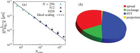
Figure 1. Parallel performance of the code on the Marconi-KNL cluster. (a) Parallel scaling of the direct numerical simulation (DNS), the elapsed time refers to a single DNS step and N is the number of resolved Fourier modes; (b) CPU time spent on each step of the forward non-uniform Fast Fourier Transform algorithm for N=1024 and on 16,384 processors. The discrete convolutions are computed on NS=4 grid points
2.3 Parallel implementation
The Eulerian–Lagrangian code is parallelized by means of the Message Passing Interface with a pencil domain decomposition. The FFTs are executed in parallel by means of the P3DFFT library [24]. Thus, the transposition of the pencils required for the three-dimensional FFT is performed by means of the MPI_Alltoall utility. Due to the Eulerian domain decom- position, the Lagrangian particles migrate through next-neighboring processes and need to be redistributed at each time step. Accordingly, the interpolation at the position of particles that are close to the borders between processors also requires communication of the fluid fields at the borders. The same communicator is employed to exchange both particle and fields at the boundary between processors by means of the MPI_Neighbor_collectives utilities. The coexistence of global and local communications is challenging for the parallel architecture and can be optimized by the accurate choice of the neighboring processors, by MPI process binding. The convolutions in physical space require a considerable amount of computational time and should be optimized. Convolutions also introduce aliasing, which is removed by padding. A 3/2 oversampling factor is employed, which is the same used to evaluate the convective terms in the DNS. As the order of the B-spline polynomials employed increases, the portion of grid points to exchange between neighboring processors becomes larger, rendering the communications more costly. The optimum values of the degree of the basis depend on the resolution, kmaxη, and does not exceed 4 for usual resolutions (kmaxη ~ 1.5), as discussed in van Hinsberg et al. [12]. Due to the compact support of the employed basis, each particle contributes to the coupling field in a limited number of grid points surrounding its position, which substantially improves the efficiency of the computation and parallelization. Also, separation of variables allows to efficiently implement the discretization of Eq. (8), providing a noticeable speed-up of the computation. An additional advantage of the B-spline basis, from the implementation viewpoint, is that its Fourier transform can be precomputed and stored, avoiding the evaluation of exponentials at each interpolation. Moreover, in three dimensions, the values of B along each coordinate can be stored separately, substantially reducing the memory requirement [18].
$\sum_{p, l, m, n} a_{p} B\left(\boldsymbol{x}_{l m n}-\boldsymbol{x}_{p}\right)=\sum_{p} a_{p} \sum_{n} B\left(z_{n}-z_{p}\right)$
$\sum_{m} B\left(y_{m}-y_{p}\right) \sum_{l} B\left(x_{l}-x_{p}\right)$
The scaling of the parallel computation on the Marconi-KNL cluster is shown in Figure 1a. The elapsed time refers to a step of the DNS, that is, the computation of a time step of Eqns. (1) and (2). The velocity and temperature fields are discretized with N3 Fourier modes, NP=(3N/2)3 particles are dispersed in the flow and the discrete convolutions are computed on NS=4 grid points. The elapsed time is normalized by the expected computational cost of the FFT and NUFFT algorithms, that is, O(N3 log2 N). The percentage of CPU time necessary for each step of the forward NUFFT is shown in Figure 1b, for 10243 Fourier modes, 15363 particles, and on 16,384 processors. The spreading step refers to the convolution in physical space, Eq. (9). The exchange step refers to the send/receive and summation of the halo regions between neighboring MPI processes. In the highly parallel computation considered, the exchange step takes a moderate amount of time with respect to the other steps. The FFT, Eq. (10), is the most expensive part of the algorithm while the projection step, Eq. (11), is the least expensive since it consists only of a multiplication.
Results of a DNS of a forced, statistically steady, homogeneous, and isotropic particle-laden turbulent flow are presented. The fluid and particle phase are two-way coupled and the parameters used in the simulations are listed in Table 1.
Table 1. Dimensionless parameters for the numerical simulations
|
Inverse Reynolds number |
v = Re-1 |
0.0025 |
|
Prandtl number |
Pr =v/κ |
1 |
|
TKE dissipation rate |
$\varepsilon$ |
0.25 |
|
Temperature fluctuation |
|
0.1 |
|
Dissipation rate |
$\chi$ |
|
|
Taylor microscale Reynolds number |
$R e_{\lambda}$ |
130 |
|
Forced wavenumber |
kf |
√2 |
|
Domain size |
L |
2π |
|
Number of Fourier modes |
N |
256 |
|
Resolution |
$k_{\max } \eta$ |
1.7 |
|
Particle/fluid density ratio |
ρp / ρf |
1000 |
|
Particle/fluid specific heat capacity ratio |
cp / cf |
4 |
|
Volume fraction |
$\varphi$ |
0.0002 |
|
Number of particles |
NP |
3343360–49136640 |
|
Stokes number |
St |
0.5, 0.75, 1, 1.5, 2, 3 |
|
Thermal Stokes number |
$S t_{\theta}$ |
6 St |
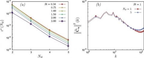
The accuracy of the computation of the particle feedback terms in Eq. (1) is critical for an accurate simulation of particle-laden flows in the two-way coupling regime. In order to assess the accuracy of the computation through NUFFT, the effect of the order of the B-spline basis on the spectral representation of the coupling terms is analyzed. Quantitative estimation of the convergence is obtained by comparing the spectrum of the coupling terms computed with B-splines of different orders,
$\varepsilon^{s}\left(N_{s}\right)=\frac{\left.\sum_{k}|| \hat{c}_{k}\right|_{N_{k}} ^{2}-\left|\hat{c}_{k}\right|_{N_{k}-1}^{2} |}{\sum_{k}\left|\hat{C}_{k}\right|_{N_{s}}^{2}}$ (12)
where, subscript NS indicates the number of points used for the discrete convolution. Figure 2a shows the relative error $\mathcal{E}^{S}$ (NS) on the momentum coupling as a function of NS for different Stokes numbers. The error introduced by a low-order basis may be too large for a DNS: NS larger than two is required to achieve an accuracy which is at least comparable with the accuracy of the time integration and spatial discretization employed in standard DNS. Moreover, regularization functions would fail to provide an accurate representation of the coupling, since this technique would cut a large amount of energy contained in the coupling field at large wave numbers, according to the chosen regularization scale. Figure 2b compares the three-dimensional spectrum of the momentum coupling for St=1 computed by NUFFT with order zero (NS=1) and order four (NS=5) B-spline basis. The two spectra noticeably differ, since the low-order polynomial overestimates the coupling energy at low wave numbers and underestimates the coupling energy at high wave numbers.
The exact Fourier representation of a generic coupling term, $C(x)=\sum_{p} a_{p} \delta\left(x-x_{p}\right)$, reads
$\overline{\hat{c}}_{k}=\sum_{p} a_{p} \exp \left(-i \boldsymbol{k} \cdot \boldsymbol{x}_{p}\right)$ (13)
and its three-dimensional discrete spectrum is
$\left|\overline{\hat{c}}_{k}\right|^{2} \sim 4 \pi \boldsymbol{k}^{2} \sum_{p} a_{p}^{2}+2 \sum_{\|k\|=k} \sum_{p} \sum_{q>p} a_{p} a_{q} \cos \left(\boldsymbol{k} \cdot\left(\boldsymbol{x}_{p}-\boldsymbol{x}_{q}\right)\right)$ (14)
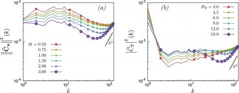
where, the number of grid points on a spherical shell of radius k is approximated with its continuum limit, 4πk2. The second term at right-hand side of Eq. (14) is related to the correlation between the positions of the particles, so that for weakly correlated particles, the first term at right-hand side of Eq. (14) dominates, thus producing a ~k2 spectrum. This trend is due to the discrete nature of the coupling term, specifically, to the interaction of the particle with itself and it gives rise to an infinite amount of spectral energy. This self-interaction contribution always dominates at large k. On the other hand, when a finite correlation exists, the second term at right-hand side of Eq. (14) dominates and, for a large number of particles, the spectrum of the particle feedback is determined by two-particle statistics. These behaviors can be seen in Figure 3, which shows the spectra of the velocity and temperature coupling, computed by means of NUFFT with a fourth-order B-spline basis. The coupling terms contain a considerable amount of energy at large wave numbers and, for large Stokes numbers, a k2 trend appears in the higher simulated wave numbers, as it has been observed in the framework of cloud microphysics [4]. The k2 trend is evident for particles with large inertia, St>1, and it extends at lower wave numbers when St increases. Indeed, the k2 trend is accentuated by the lack of correlation between particle pairs, Eq. (14), which is the case of particles with large inertia. The next section deals with the possible removal of the particle self-interaction.
Figure 2. Convergence of the forward non-uniform Fast Fourier Transform. (a) Convergence of the spectral representation of the momentum coupling quantified by the relative error εs and (b) effect of the order of the basis on the momentum coupling spectrum
Figure 3. Spectra of the coupling terms, obtained by means of the forward NUFFT with NS=5. (a) Momentum coupling and (b) temperature coupling
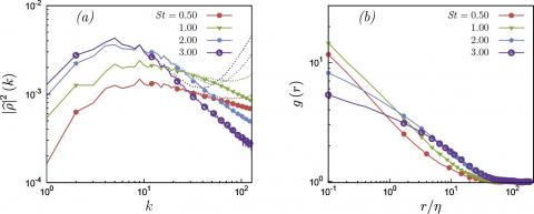
Figure 4. Inertial particle clustering observed in Fourier and in physical space. (a) Three- dimensional corrected spectra (solid) and bare spectra (dotted line) of the particle mass distribution. (b) Radial distribution function for different particle inertia
3.2 Spectral representation of the particle phase
Two-particle statistics can be efficiently characterized in Fourier space through NUFFT, since the NUFFT allows to get an accurate representation of the particle phase as a continuum field, so as to determine the density, momentum, and temperature of the particle distribution. Particle mass density and velocity fields are useful to quantify the particle clustering [25]. From the discrete particle distribution, the particle phase density is
$\rho(x, t)=\sum_{p} m_{p} \delta\left(x-x_{p}(t)\right.$,
where, $m_{p}=4 \rho_{p} \pi r_{p}^{3}$ is the single-particle mass. Since the particles are monodisperse, in these simulations, then mp=m. The discrete particle mass distribution is smoothed by means of B-splines and represented in physical space on a Cartesian grid:
$\tilde{\rho}(\boldsymbol{x}, t)=m \sum_{p} B\left(\boldsymbol{x}-\boldsymbol{x}_{p}(t)\right)$. (15)
The smoothed field is transformed by means of FFT and the convolution is removed in Fourier space. Therefore, the spectrum of the particle density field can be obtained as
$|\hat{\rho}(\boldsymbol{k}, t)|^{2}=\frac{1}{(2 \pi)^{6}} \sum_{\|\boldsymbol{k}\|=\boldsymbol{k}}\left|\frac{F[\tilde{\rho}](\boldsymbol{k}, t)}{F[B](\boldsymbol{k})}\right|^{2}$ (16)
where, the denominator removes the B-spline regularization and ensures that the mean value of ρ is equal to $\rho_{p} \varphi$, that is, $\hat{\rho}(0, t)=\rho_{p} \varphi$. Eq. (16) provides the NUFFT approximation to the discrete reference spectrum of (15), which is
$|\hat{\rho}(\boldsymbol{k}, t)|_{r}^{2} \sim \frac{m^{2}}{(2 \pi)^{6}}\left[4 \pi k^{2} N_{P}+2 \sum_{\|\boldsymbol{k}\|=k} \sum_{p} \sum_{q>p} \cos \left(\boldsymbol{k} \cdot\left(\boldsymbol{x}_{q}(t)-\boldsymbol{x}_{p}(t)\right)\right)\right]$ (17)
The ~k2 trend is removed from the NUFFT approximation of the spectrum, Eq. (16), using the expression of the exact spectrum, Eq. (17),
$|\hat{\rho}(\boldsymbol{k}, t)|_{c}^{2}=\frac{1}{(2 \pi)^{6}}\left[\sum_{\|\boldsymbol{k}\|=k}\left|\frac{F[\tilde{\rho}](\boldsymbol{k}, t)}{F[B](\boldsymbol{k})}\right|^{2}-4 \pi k^{2} N_{p} m^{2}\right]$ (18)
to obtain a corrected spectrum.
The spectra of the particle mass distribution field, for different particle inertia, are shown in Figure 4a. The solid lines represent the corrected spectrum, defined by Eq. (18), while the dotted lines refer to the bare spectrum, defined in Eq. (16). In the lower wave number range, the two spectra coincide; they begin to differentiate as soon as particle inertia is able to decor- relate particle motions. Therefore, the threshold wave number at which this happens reduces as the Stokes number is increased. The slope of the spectrum gives an indication of particle clustering, with lower slopes produced by the sharpening of particle concentration fronts [25], which is maximum at St=O (1). The slope of the spectra at large wave numbers is well above −3, that is, the value corresponding to the square-integrable gradient of the particle density field. Thus, the particle density field displays fronts for finite particle inertia [25]. The particle density field encloses features which can be characterized in physical space by means of the radial distribution function (RDF). The RDF is defined as the ratio between the number of particles Nr which lie on a spherical shell of radius r and the average number of particles expected on the shell for a uniform particle distribution [26]:
$g(r)=\frac{\Omega}{N_{p}} \lim _{\delta r \rightarrow 0} \frac{N_{r}(\delta r)}{4 \pi r^{2} \delta r}$ (19)
where, $\Omega$ is the volume of the whole domain. The RDF, for different particle inertia, is shown in Figure 4b. Fluid particles, for which St=0, are uniformly distributed in the domain so that g(r)=1. As the Stokes number is increased, particles tend to agglomerate at small separation, and this small-scale clustering is maximum at St=O(1). As the Stokes number is further increased, the clustering strength reduces and the particle distribution tends to be uniform again. The RDF directly provides information about clustering using physical space quantities only. Remarkably, an equivalent description of clustering can be carried out by means of the corrected spectra of the particle mass distribution equivalent field. In fact, at large wave number, the spectrum of the particle mass distribution increases with St up to St=O(1) and then decreases. This coincides with the trend of the RDF at small separation. Notice that the information about small-scale clustering is not evident from the bare spectra since it is concealed by the k2 trend. The spectral analysis of the particle mass distribution by means of the equivalent field shows that the NUFFT can be employed to characterize two-particle statistics in a simpler manner than the challenging direct computation in physical space.
Particle equivalent fields for the particle velocity and temperature allow to draw a similarity between the spectral representation of the particle phase and the particle structure functions. The smoothed equivalent particle velocity and temperature fields are defined as,
$\begin{aligned} \tilde{v}(\boldsymbol{x}, t) &=\frac{\sum_{p} m_{p} v_{p}(t) B\left(\boldsymbol{x}-\boldsymbol{x}_{p}(t)\right)}{\sum_{p} m_{p} B\left(\boldsymbol{x}-\boldsymbol{x}_{p}(t)\right)}, \\ \tilde{\theta}(\boldsymbol{x}, t) &=\frac{\sum_{p} m_{p} c_{p} \theta_{p}(t) B\left(\boldsymbol{x}-\boldsymbol{x}_{p}(t)\right)}{\sum_{p} m_{p} c_{p} B\left(\boldsymbol{x}-\boldsymbol{x}_{p}(t)\right)} \end{aligned}$, (20)
so that particle momentum and enthalpy per unit volume are $\tilde{\rho} \tilde{v}$ and $\tilde{\rho} c_{p} \tilde{\theta}$. The equivalent velocity and temperature field definition take into account that several particles could be located around each grid point. For St=0 and St=0, these equivalent fields coincide with the fluid velocity and temperature fields because velocity and temperature are equal to the fluid velocity and temperature and particles are uniformly distributed. As for the particle density field, the particle velocity and temperature smoothed fields can be transformed by means of FFTs. Figure 5 shows the spectra of the particle velocity and temperature equivalent fields. An inertial range can be identified in the particle velocity and temperature equivalent fields spectra. However, this observation is only qualitative, since a higher Reynolds number would be required to observe a well-developed inertial scaling. The trend of the particle velocity spectrum is close to the Kolmogorov scaling at low Stokes numbers. In fact, particles with low inertia tend to behave like the underlying fluid particles. As the Stokes number increases, the slope of the spectrum in the inertial range decreases; indeed, particles tend to spatially decor- relate and the bare momentum spectrum approaches a k2 trend as seen above. The energy of the particle velocity and temperature fluctuations decreases with the particle inertia, which is evident at the largest scales. At small scales, the k2trend, not removed in the figure, is not as evident as for the coupling terms. The spectra of the continuum equivalent temperature present a larger deviation from the Obukhov scaling because the thermal Stokes number is always much larger than the Stokes number in the simulations since Stθ=6St is chosen in order to emulate water droplets in the air. Thus, even at the smallest Stokes number, the behavior of the particle temperature is much different than the underlying fluid temperature. This larger thermal Stokes number, which corresponds to larger thermal relaxation time, produces a large memory effect along particle paths so that they are more sensible to large scale fluctuations and their statistics can be affected by the details of the large-scale forcing. Moreover, these deviations from the Obukhov scaling can also be attributed to the high intermittency of the advected passive scalars like temperature and to the tendency of particles to cluster in the regions of large temperature gradients [18]. These may be some of the reasons behind the deviation of the spectrum of the equivalent temperature field from the classical Obukhov scaling.
3.3 Scale by scale analysis
Inertial particles modify the fluid flow fluctuations across all the scales of the flow through the coupling terms in Eq. (1). This effect of particles on the flow can be quantified through the second-order longitudinal velocity and temperature structure functions, which are defined as:
$S_{u \|}^{2}(r)=\left\langle\left(\delta_{r} u \cdot \hat{\boldsymbol{r}}\right)^{2}\right\rangle, S_{T}^{2}(\boldsymbol{r})=\left\langle\left(\delta_{\boldsymbol{r}} T\right)^{2}\right\rangle$
where, $\langle\cdot\rangle$ indicates the ensemble average, $\delta_{r} u$ is the velocity increment computed at separation r, $r=\|r\|$ and $\hat{\boldsymbol{r}}=\boldsymbol{r} / r$ is the unit vector in the direction of the separation vector.
Figure 6 shows the second-order longitudinal fluid velocity structure functions and fluid temperature structure function, for different inertia of the suspended particles. The statistics are non-dimenwsionalized by means of a small-scale velocity fluctuation $u_{\eta}=(\varepsilon v)^{1 / 4}$ and a small-scale temperature fluctuation $\theta_{\eta}=\chi^{1 / 2}(\kappa / \varepsilon)^{1 / 4}$ . The fluctuations of the fluid velocity field are modulated by the suspended inertial particles at all the scales. At the smallest scales the second-order structure functions always decrease due to the presence of particles, and the reduction is more evident as the particle inertia is increased. At small separation, the second-order structure function is proportional to the dissipation rate of turbulent kinetic energy (TKE) due to the fluid velocity gradients, that is, $S_{u \|}^{2} \propto\|\nabla u\|^{2}, r \leq \eta$. Thus, the contribution to the dissipation rate by the interaction with the particles increases monotonically with particle inertia, at the energy injection rate maintained constant. A qualitative similar behavior can be observed in the fluid temperature structure function.
At a separation larger than the integral length scale l, the second-order structure function is proportional to the variance of the fluctuations of the velocity field, that is, $S_{u \|}^{2} \propto u^{\prime 2}, r \leq l$. These results show that the TKE decreases as the particle inertia is increased. However, in this scale range, the fluid temperature field displays a qualitatively different behavior. In fact, the suppression of the fluid temperature fluctuations by the suspended inertial particles appears to have a maximum because particles with a relaxation time much larger than fluid time scales become less and less effective in the large-scale modulation of the fluid temperature fluctuations [27]. The most effective Stokes number for large-scale fluctuations suppression may depend on the Reynolds and Prandtl numbers and deserves further investigation.
Figure 7 shows the second-order longitudinal particle velocity structure function and particle temperature structure function, for different particle inertia. At small separation, as the Stokes number is increased, the second-order particle velocity and temperature structure functions noticeably deviate from the r2behavior, that is, the behavior expected for an ana- lytic field. Pairs of particles that are very close to each other have on average much larger relative velocity than the corresponding fluid particles [10]. At intermediate-large scales, the particle velocity and temperature second-order structure functions exhibit a $r^{2 / 3}$ trend [26] which is consistent with the inertial range scaling of the particle velocity and temperature spectra in Figure 5. At large separation, the energy of the particle velocity and temperature fluctuations always decreases increasing the particle inertia, for Stokes numbers large enough. This is consistent with the reduction of the particle velocity and temperature spectral energy (Figure 5). However, due to the large inertia, small particle velocity and temperature fluctuations correspond to relatively large fluctuations of momentum and thermal energy. The particle velocity and temperature structure functions show qualitatively similar behavior, even though the thermal Stokes number of the particles is quite larger than the dynamic particle Stokes number, rendering the thermal caustics and filtering more evident. A detailed examination of the temperature modulation due to inertial particles in turbulence can be found in Carbone et al. [27].
Figure 5. Spectra of the particle equivalent fields for different particle inertia. (a) Spectrum of the particle velocity equivalent field. (b) Spectrum of the particle temperature equivalent field
Figure 6. Second-order structure functions of fluid velocity and temperature in the two-way coupling regime, for various inertia of the suspended particles. (a) Longitudinal fluid velocity structure functions. (b) Fluid temperature structure functions
Figure 7. Second-order structure functions of particle velocity and temperature in the two- way coupling regime, for various particle inertia. (a) Longitudinal particle velocity structure functions. (b) Particle temperature structure functions
In this work, the ability of the NUFFT to allow accurate simulation of particle-laden turbulent flows has been explored. The NUFFT with B-spline basis turned out to be an effective tool for the numerical simulation of particle-laden flows in the two-way coupling regime. Also, the NUFFT allows for the spectral representation of the particle phase by means of equivalent fields, which can be employed to characterize two-particle statistics. It is shown that particle clustering can be described in detail by means of the particle mass distribution equivalent field, obtained by NUFFT. Also, analogies can be drawn between the particle second-order structure functions and the spectra of the particle velocity and temperature equivalent fields. The ability to easily obtain equivalent particle fields is an interesting feature of the NUFFT which looks promising to compute multiple particle statistics from DNS of particle-laden flows.
The authors would like to thank Dr. A. D. Bragg for fruitful discussions on the topic. The authors acknowledge the computer resources provided by LaPalma Supercomputer at the Instituto de Astrofisica de Canarias through the Red Espanola de Supercomputacion (project FI-2018-1-0044) and by CINECA under the ISCRA initiative, project HP10CWVISL. Additional resources provided by HPC@POLITO (http://www.hpc.polito.it).
[1] Zonta, F., Marchioli, C., Soldati, A. (2008). Direct numerical simulation of turbulent heat transfer modulation in micro-dispersed channel flow. Acta Mechanica, 195(1-4): 305-326. https://doi.org/10.1007/s00707-007-0552-7
[2] Ravnik, J., Marchioli, C., Soldati, A. (2018). Application limits of Jeffery’s theory for elongated particle torques in turbulence: A DNS assessment. Acta Mechanica, 229(2): 827-839. https://doi.org/10.1007/s00707-017-2002-5
[3] De Lillo, F., Cencini, M., Durham, W.M., Barry, M., Stocker, R., Climent, E., Boffetta, G. (2014). Turbulent fluid acceleration generates clusters of gyrotactic microorganisms. Physical Review Letters, 112: 044502. https://doi.org/10.1103/PhysRevLett.112.044502
[4] Saito, I., Gotoh, T. (2018). Turbulence and cloud droplets in cumulus clouds. New Journal of Physics, 20(2): 023001. https://doi.org/10.1088/1367-2630/aaa229
[5] Elghobashi, S. (1991). Particle-laden turbulent flows: Direct simulation and closure models. Applied Scientic Research, 48(3): 301-314. https://doi.org/10.1007/BF02008202
[6] Cui, Y., Ravnik, J., Hribersek, M., Steinmann, P. (2018). On constitutive models for the momentum transfer to particles in fluid-dominated two-phase flows. Springer Inter- national Publishing: Cham, pp. 1-25. https://doi.org/10.1007/978-3-319-70563-7_1
[7] Maxey, M.R. (1987). The gravitational settling of aerosol particles in homogeneous turbulence and random flow fields. Journal of Fluid Mechanics, 174: 441-465. https://doi.org/10.1017/S0022112087000193
[8] Bragg, A.D., Collins, L.R. (2014). New insights from comparing statistical theories for inertial particles in turbulence: I. Spatial distribution of particles. New Journal of Physics, 16(5): 055013. https://doi.org/10.1088/1367-2630/16/5/055014
[9] Dhariwal, R., Bragg, A.D. (2018). Small-scale dynamics of settling, bidisperse particles in turbulence. Journal of Fluid Mechanics, 839: 594-620. https://doi.org/10.1017/jfm.2018.24
[10] Wilkinson, M., Mehlig, B. (2005). Caustics in turbulent aerosols. Europhysics Letters, 71(2): 186-192. https://doi.org/10.1209/epl/i2004-10532-7
[11] van Hinsberg, M.A.T., ten Thije Boonkkamp, J.H.M., Toschi, F., Clercx, H. (2012). On the efficiency and accuracy of interpolation methods for spectral codes. SIAM Journal on Scientific Computing, 34(4): B479-B498. https://doi.org/10.1137/110849018
[12] van Hinsberg, M.A.T., ten Thije Boonkkamp, J.H.M., Toschi, F., Clercx, H. (2013). Optimal interpolation schemes for particle tracking in turbulence. Physical Review E, 87(4): 043307. https://doi.org/10.1103/PhysRevE.87.043307
[13] Zamansky, R., Coletti, F., Massot, M., Mani, A. (2014). Radiation induces turbulence in particle-laden fluids. Physics of Fluids, 26(7). https://doi.org/10.1063/1.4890296
[14] Pan, Y., Banerjee, S. (1996). Numerical simulation of particle interactions with wall turbulence. Physics of Fluids, 8(10): 2733-2755. https://doi.org/10.1063/1.869059
[15] Greengard, L. (1988). The Rapid Evaluation of Potential Fields in Particle Systems. MIT Press.
[16] Lindbo, D., Tornberg, A.K. (2011). Spectral accuracy in fast Ewald-based methods for particle simulations. Journal of Computational Physics, 230(24): 8744-8761. https://doi.org/10.1016/j.jcp.2011.08.022
[17] Gualtieri, P., Picano, F., Sardina, G., Casciola, C.M. (2015). Exact regularized point particle method for multiphase flows in the two-way coupling regime. Journal of Fluid Mechanics, 773: 520-561.
[18] Carbone, M., Iovieno, M. (2018). Application of the non-uniform fast fourier transform to the direct numerical simulation of two-way coupled turbulent flows. WIT Transactions on Engineering Sciences, 120: 237-248.
[19] Maxey, M.R., Riley, J.J. (1983). Equation of motion for a small rigid sphere in a nonuniform flow. Physics of Fluids, 26(4): 883-889. https://doi.org/10.1063/1.864230
[20] Hochbruck, M., Ostermann, A. (2010). Exponential integrators. Acta Numerica, 19: 209-286. https://doi.org/10.1017/S0962492910000048
[21] Kumar, B., Schumacher, J., Shaw, R.A. (2013). Cloud microphysical effects of turbulent mixing and entrainment. Theoretical and Computational Fluid Dynamics, 27(3): 361-376. https://doi.org/10.1007/s00162-012-0272-z
[22] Beylkin, G. (1995). On the Fast Fourier Transform of functions with singularities. Applied and Computational Harmonic Analysis, 2(4): 363-381. https://doi.org/10.1006/acha.1995.1026
[23] Sundaram, S., Collins, L.R. (1996). Numerical considerations in simulating a turbulent suspension of finite-volume particles. Journal of Computational Physics, 124(2): 337-350. https://doi.org/10.1006/jcph.1996.0064
[24] Pekurovsky, D. (2012). P3DFFT: A framework for parallel computations of Fourier transforms in three dimensions. SIAM Journal on Scientific Computing, 34(4): C192-C209. https://doi.org/10.5281/zenodo.2634590
[25] Boffetta, G., Celani, A., Lillo, F.D., Musacchio, S. (2007). The Eulerian description of dilute collisionless suspension. Europhysics Letters, 78(1): 14001. https://doi.org/10.1209/0295-5075/78/14001
[26] Ireland, P.J., Bragg, A.D., Collins, L.R. (2016). The effect of Reynolds number on inertial particle dynamics in isotropic turbulence. Part 1. Simulations without gravitational effects. Journal of Fluid Mechanics, 796: 617-658. https://doi.org/10.1017/jfm.2016.238
[27] Carbone, M., Bragg, A.D., Iovieno, M. (2019). Multiscale fluid-particle thermal interaction in isotropic turbulence. Journal of Fluid Mechanics, 881: 679-721. https://doi.org/10.1017/jfm.2019.773