Chun Chen | Bin Yang | Qiong Wu* | Bingjie Dong
© 2020 IIETA. This article is published by IIETA and is licensed under the CC BY 4.0 license (http://creativecommons.org/licenses/by/4.0/).
OPEN ACCESS
The accurate output efficiency measurement is of great significance for improving the output efficiency of industrial parks. The evaluation results of existing related studies are prone to errors due to the neglect of the interference of environment factors and random factors. To reduce such deficiency, this paper combined DEA (Data Envelopment Analysis) with SFA (Stochastic Frontier Approach) under the framework of production function, and employed a three-stage DEA model to measure the output efficiency of provincial-level industrial parks in Hubei province China after the influence of non-production factors such as local economic factors and random factors had been excluded. The research results showed that compared with single-stage DEA, the measurement results of three-stage DEA were more reasonable. On the whole, the output efficiency of industrial parks in various regions of Hubei was relatively low, only a few industrial parks in Wuhan, Ezhou, Xianning and Xiantao were at the frontier of effective efficiency; in 16 prefecture-level cities of Hubei province, more than half of the industrial parks were in the stage of Returns To Scale (RTS) increase; in terms of Pure Technical Efficiency (PTE), the differences among various regions were not much, and there’s PTE>Scale Efficiency (SE) > Technical Efficiency (TE), indicating that improving the technical efficiency is the key to improving the output efficiency of industrial parks.
industrial park, output efficiency, three-stage DEA
China is facing the problems of overcapacity and industrial transformation and upgrading, and incompetent products and insufficient output efficiency have become obstacles hindering the transformation and development of China’s industrial industry. Industrial parks are the prime engines for local economic growth, and how to accurately and quantitatively measure their output efficiency and find out the key influencing factors are problems demanding prompt solutions in the process of regional industrial transformation and upgrading. Hubei Province is located at the core area of the Central Plains connecting the east and west China, and the research on the measurement of the output efficiency of industrial parks in Hubei is conductive to promoting the economic development and industrial transformation of Hubei province. In addition, the research is also of great significance to promote the development of neighbor provinces and the "Yangtze River Economic Belt".
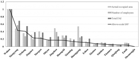
According to the data from the Hubei Provincial Bureau of Statistics, as of the first half of 2018, there were 132 industrial parks (high-tech zones, development zones) in Hubei Province, among which there’re 119 provincial-level industrial parks, and these parks have become the main force for the economic development of Hubei province. For industrial parks of comparable scale in various regions of Hubei, after their data such as the occupied area, number of employees, fixed asset investment (FAI) and above-scale industrial added value (IAV) had been subject to linear normalization, it was found that, for industrial parks in Jingmen, Xiaogan, Jingzhou, and Huangshi, the indicator of occupied areas was 0.35, 0.4, 0.5, and 0.35, respectively, while the indicator of above-scale IAV showed a downward trend. There’s deviation between the occupied area and the output value, and such deviation had happened to about half of the industrial parks in the target regions; for most of them, there’re also similar situations such as the output value had also deviated from the employee number and the FAI. Therefore, the promotion of regional industrial development does not necessarily depend on the input of production factors in a region, and only by accurately and quantitatively measuring the output efficiency of the industrial parks and analyzing the deeper reasons of their low efficiency can we improve the output efficiency of the industrial parks and promote the development of regional industrial economy (see Figure 1).
Figure 1. Production factor input of industrial parks in target regions
Industrial parks are the important economic carriers for the development of local industries, and the research on their efficiency calculations has always been valued by the academic circles. To calculate the output efficiency of industrial parks, domestic and foreign scholars mainly adopted the DEA, a non-parametric method for their studies, Tone et al. had all employed this method in efficiency measurement [1-5]. Tone’s research proved the effectiveness of DEA as an efficiency measurement tool and it’s compatible with other efficiency measurement methods. Oggioni et al. applied DEA to calculate the ecological output efficiency of the cement industry in 21 countries, and pointed out the direction for improving the efficiency of the cement industry. Domestic scholars mainly used quantitative methods to measure production efficiency, such as the linear regression had long been employed to study the output efficiency of industrial parks from multiple aspects such as constructing index systems, determining index weights, defining the ideal values of indexes and calculating the efficiency scores after environment factors have been excluded, etc. Moreover, some scholars also have calculated the output efficiency of industrial parks in certain provinces, and their calculated methods were mainly the linear regression models of Solow residuals or the single-stage DEA. One example is Shi Jiangang's research, he applied the DEA-Malmquist method to calculate the land output efficiency of industrial parks in the Yangtze River Delta, and his research results showed that the technical factors are the main factors restricting the improvement of land output efficiency. Besides, scholars also used hierarchical linear models, fuzzy integral models, multi-index comprehensive evaluations and machine learning models to calculate the output efficiency of industrial parks.
In summary, the research on the measurement of the efficiency of industrial parks had achieved rich results, but there are still a few deficiencies: (1) Most existing studies only measured the efficiency of industrial parks in a certain area, and there’s no horizontal comparison between their efficiency values; (2) In terms of the usage method, the efficiency values calculated by single-stage DEA include the influence of non-production factors such as random factors and environment factors, while the efficiency values calculated by linear models or other evaluation models have certain deviations due to the randomness existing in the process of index weight assignment; (3) In terms of the research on the efficiency of industrial parks, output efficiency is insufficiently studied, the land resource is an important production factor, but its effect can only be exerted when it is closely combined with other production factors such as labor, capital and technology; but due to the poor availability of industrial park data, most existing studies only focused on the output efficiency of land, therefore, the obtained efficiency values had artificial selection biases.
Targeting at the problems summarized above, this paper focuses on the accurate measurement of the output efficiency of industrial parks in various regions; the innovations of this research are: (1) research data: this research had comprehensively collected data of provincial-level industrial parks such as the land use, labor force, capital and input, etc.; and it matched the industrial parks data with the external environmental data of the regions; (2) research method: this research combined with production function and three-stage DEA to calculate and study the output efficiency of the industrial parks in Hubei Province, its superiority lies in that it had included the land factor in the framework of the production function to avoid index selection bias [6-10]; (3) efficiency measurement using three-stage DEA does not require manual selection of index weights; it can eliminate the influence of non-production factors on the output efficiency, and can make horizontal comparisons of the output efficiency of industrial parks in multiple regions.
The structure of below sections is: the second part is model construction and variable selection; the third part is empirical analysis; the fourth part is conclusions and suggestions.
2.1 Model construction
DEA is a non-parametric technical efficiency analysis method based on the comparison of evaluated objects. The method is able to assign weight values objectively, and analyze the influencing factors of the decision-making units (DMUs), and there’s no need to determine the input-output function relationship in advance; the method has good objectivity in multiple input and output evaluations; therefore, it is a mainstream method of efficiency analysis [11-15].
According to the efficiency measurement method, DEA models can be divided into input-oriented model, output-oriented model and non-oriented model. The input-oriented DEA model measures the degree of inefficiency of the evaluated units from the perspective of input, it focuses on the decrement of input that should be reduced when the technical efficiency has been reached under the condition that the output is not reduced. The output-oriented model evaluates the degree of inefficiency of each unit from the perspective of output, it focuses on the increment of output that should be increased when technical efficiency has been reached under the condition that the input is not increased. The non-oriented model measures the efficiency of the evaluated units from both aspects of input and output. Based on the research purpose of this paper that it aims to improve the efficiency of inefficient units by reducing input, the input-oriented model had been chosen in this paper [16-20].
The assumptions of the input-oriented model are: the production sector has fixed RTS, multiple input elements, constant output, and the isoquant curve and isocost curve of per unit output have a point of tangency. When the output efficiency is measured by the single-stage DEA, the efficiency not only reflects the effectiveness of management in the unit individual, but also includes the influence of random factors and environment factors (regional economic environment and policy environment). To eliminate the influence of non-production factors on the output efficiency, Fried et al. had proposed the three-stage DEA model [21]. This paper divided the panel data of multiple years into cross-section data, and performed three-stage DEA on the cross-section data of each year. The construction method of the three-stage DEA model in this paper is:
First stage: the input-oriented BCC (Banker-Charnes-Cooper) model was employed to perform DEA on the historical data of industrial parks of Hubei province. Assuming that there are n prefecture-level cities, m input terms, s output terms, DMU0 represents any DMU, then the set of production techniques of the industrial parks is:
$T=\left\{(x, y): x \in R^{m+} ; y \in R^{s+}\right\}$,
where, x is the input, y is the output; there are: $x=\left(x_{1}, x_{2}, \ldots, x_{n}\right) \in R^{m+}, y=\left(y_{1}, y_{2} \ldots, y_{n}\right) \in R^{s+}$. The programming formulas of the input-oriented BCC model are:
$\min \theta$
s.t. $\sum_{j=1}^{n} \lambda_{j} x_{i j} \leq \theta x_{i k}$
$\sum_{j=1}^{n} \lambda_{j} y_{r j} \leq \theta y_{i k}$
$\sum_{j=1}^{n} \lambda_{j}=1,(\lambda \geq 0)$
$i=1,2, \ldots m, r=1,2, \ldots q, j=1,2, \ldots n$
The dual programming formulas are:
$\max \sum_{r=1}^{s} \mu_{r} y_{r k}-\mu_{0}$
s.t. $\sum_{r=1}^{q} \mu_{r} y_{r j}-\sum_{i=1}^{m} v_{i} x_{i j}-\mu_{0} \leq 0$
$\sum_{i=1}^{m} v_{i} x_{i j}=1$
$v \geq 0 ; \mu \geq 0 ; \mu_{0}$ is an arbitrary value
$i=1,2, \ldots m, r=1,2, \ldots q, j=1,2, \ldots n$
The efficiency of BCC model under the VRS (Variable Returns-to-Scale) condition is called the Technical Efficiency (TE); the efficiency under the CRS (Constant Return to Scale) condition is called the Pure Technical Efficiency (PTE); the Scale Efficiency (SE) of the BCC model is the ratio of TE and PTE.
Second stage: SFA was adopted to analyze the slack values of the first stage and adjust the input and output. The slack values of each DMU obtained in the first stage were the differences after compared with the input/output ratios of DMUs at the frontier of efficiency, and such differences were affected by the joint influence of management factors, random factors and environment factors. Therefore, SFA was used to analyze the slack values of the first stage so as to improve the reliability of DEA estimation. Assuming that there are q observable external environment variables, then, the SFA equation can be expressed as:
$s_{i k}=f^{i}\left(Z_{k} ; \beta^{i}\right)+v_{i k}+u_{i k}$,
where, i=1, 2, ..., m, represents the i-th input; k=1, 2, ..., n, represents the k-th DMU; sik is the slack variable of the i-th input of the k-th DMU; zk is the observable environment variable of the k-th DMU; $\beta^{i}$ is the parameter to be estimated; generally, it takes $f(\cdot)$ to represent the influence of the environment variables on the slack variables of the i-th input, $f(\cdot)=z_{k} \beta^{i}$, vik is the stochastic disturbance term; $v_{i k} \sim N\left(0, \sigma_{v i}^{2}\right)$; uik represents management inefficiency, it conforms to truncated normal distribution or half-normal distribution, $u_{i k} \sim N\left(u^{i}, \sigma_{u i}^{2}\right)$; vik and uik are mutually independent and uncorrelated, their joint term vik+uik represents the mixed error; $\gamma=\frac{\sigma_{u i}^{2}}{\sigma_{u i}^{2}+\sigma_{v i}^{2}}$ is the proportion of the variance of management inefficiency in the total variance, and its value indicates the influence of management factors or random factors. When $\gamma \rightarrow 1$, it means that the management factors dominate the influence; when $\gamma \rightarrow 0$, the random factors dominate the influence. Based on the SFA of slack variable, the initial input of each unit was adjusted as follows:
$\hat{x_{i k}}=x_{i k}+\left[\max _{k}\left\{Z_{K} \hat{\beta}^{i}\right\}-Z_{k} \hat{\beta}^{i}\right]+\left[\max \left\{\hat{v_{i k}}\right\}-\hat{v_{i k}}\right]$.
In above formula, the first bracket represents output increment when the external environment of all units has been adjusted to the optimum; and the second bracket represents the adjustment of the random error of the input. The meaning of this formula is the initial input after environment adjustment and random error adjustment, that is to say, each DMU has the same economic environment and the same level of luckiness.
Third stage: the DEA model was used again to analyze the efficiency of the input and output after the adjustment of SFA. The efficiency values of the BCC model under CRS and VRS conditions were still adopted here. At this time, the influence of environment factors and random factors had been eliminated, so the efficiency values can reflect the management efficiency of the industrial parks more accurately.
2.2 Variable description
Due to the different levels of industrial parks, there’s heterogeneity among these parks. If they are put together to make comparisons, there might be large errors in the calculation results. Besides, the provincial-level industrial parks have become the main force of regional economic development, therefore, analyzing the provincial-level industrial parks is of greater practical significance.
Description of input and output variables: according to the basic production function in economics: $Q=f(l ; t ; c ; L)$; l represents the number of laborers; t represents technology; c represents capital input; L represents land use; Q represents output. In this paper, the number of laborers l was measured by the number of employees in the industrial parks; technology t adopted the current-year technology investment as the proxy variable, generally, it’s believed that the regional technical level and the use of new technologies in the region are positively correlated with the technology investment of the region; the capital input c was measured with the total FAI as the proxy variable, and this method is adopted in most studies; the land use L was measured by the actual occupied area of the industrial parks; the output Q was measured by the IAV of provincial industrial parks in the region.
Description of environment variables: according to the "separation hypothesis" proposed by Simar and Wilson [22], the characteristics of external environment variables are: the variables have a significant impact on the input and output efficiency of the industrial parks, and they can hardly be controlled or changed by each individual DMU. In terms of the selection of the environment variables that can affect the input of industrial parks, this paper took tax policy, social consumption level, degree of openness, technical innovation ability, regional industrial structure and public facilities and services as the environment variables of the region. The proportion of tax revenue of the industrial parks to the GDP was used to measure the tax policy of the region; the social consumption level was measured by the total retail sales of social consumption; the degree of openness was measured by the proportion of direct foreign investment and total exports in the GDP; the technical innovation ability was measured by the number of patents of the region; the regional industrial structure was measured by the proportion of the primary and tertiary industries in the total output of the region; the public facilities and services was measured by the proportion of basic infrastructure investment and public budget expenditures in the GDP. As non-production factors, the above-mentioned variables also have an impact on the output of the industrial parks; with tax policy, degree of openness, public facilities and services as examples, for the policy-type exogenous variables and the social-economic type factors, the basic logic of their impact on the output of industrial parks lies in that, non-production factors can always be combined with production factors in a certain way to promote the output of industrial parks [23] (see Table 1).
Table 1. Input-output indexes and environment indexes
|
Objective layer |
Criterion layer |
Alternative (Index) layer |
|
Output efficiency |
Input indexes |
Number of laborers; technical level; land use; capital investment |
|
Environment indexes |
Tax policy; degree of openness; social consumption level; technical innovation ability Regional industrial structure; public facilities and services |
|
|
Output indexes |
Sum of IAVs of industrial parks |
3.1 Variable description
Table 2 gives the main production variables of industrial parks and their statistical characteristics. In terms of technology, there’re large differences among various regions, and the differences were increasing year by year, the range of technology grew from 239.93 in 2013 to 406.90 in 2015; in terms of labor, the differences of labor among various regions were relatively stable, and the changes were not much; in terms of land use, the land use showed a gradual increase over the years, and the range of land use showed gradual expansion, indicating that the prefecture-level government had also increased their land use of industrial parks, and the differences of land use among different regions were increasing; in terms of capital, the differences over time were relatively stable, but the differences among different regions were relatively large; in terms of output of industrial parks, the output value showed an increasing trend year by year, and the differences among different regions also showed an expanding trend. Overall speaking, the regional differences in the input and output of industrial parks in Hubei Province were obvious, and such differences showed a trend of increasing over time.
Table 2. Statistics of variables
|
|
Minimum |
First quantile |
Median |
Mean |
Third quantile |
Maximum |
|
Technology 2013 |
25.67 |
41.84 |
70.76 |
97.28 |
143.1 |
265.6 |
|
Labor 2013 |
3.530 |
9.705 |
17.15 |
24.94 |
31.18 |
105.7 |
|
Land 2013 |
15.00 |
46.66 |
93.00 |
109.2 |
163.8 |
380.4 |
|
Capital 2013 |
44.51 |
148.8 |
312.9 |
475.2 |
536.7 |
1637.7 |
|
Output 2013 |
164.4 |
278.3 |
481.7 |
741.4 |
601.9 |
3859 |
|
Technology 2015 |
5.550 |
122.3 |
204.1 |
207.6 |
276.9 |
569.6 |
|
Labor 2015 |
5.770 |
10.31 |
20.23 |
24.02 |
24.33 |
104.1 |
|
Land 2015 |
23.90 |
45.52 |
97.55 |
114.8 |
150.3 |
333.7 |
|
Capital 2015 |
142.7 |
219.4 |
561.3 |
651.4 |
787.5 |
1847 |
|
Output 2015 |
185.8 |
31.60 |
531.3 |
812.8 |
647.9 |
4785 |
|
Technology 2017 |
9.902 |
75.57 |
129.7 |
156.5 |
223.9 |
416.8 |
|
Labor 2017 |
5.610 |
11.27 |
22.43 |
29.09 |
30.27 |
118.5 |
|
Land 2017 |
26.41 |
59.48 |
137.8 |
159.4 |
224.5 |
531.6 |
|
Capital 2017 |
150.4 |
289.0 |
787.2 |
919.2 |
1138 |
3014 |
|
Output 2017 |
239.0 |
384.6 |
667.8 |
1015 |
764.7 |
5227 |
Note: data source is Hubei Provincial Statistical Yearbook
3.2 Empirical analysis of three-stage DEA
The empirical study was completed on R3.3.1. According to the model building steps, the efficiency of industrial parks in various regions of Hubei Province was analyzed one by one. First, single-stage DEA was performed on the efficiency of industrial parks, the values of efficiency and RTS are shown in Table 3.
In terms of TE, the coefficient of variation increased from 0.276 to 0.302, and the differences among regions showed a gradual increase trend; the mean values of TE were between 0.692 and 0.776; and the TE values of most regions were in a state of inefficiency.
In terms of PTE, the differences among regions also showed gradual increase over the years, and the coefficient of variation increased from 0.214 to 0.296; and most regions were in the state of inefficiency as well.
In terms of SE, the differences among regions were relatively stable. From 2015 to 2017, the coefficient of variation decreased, indicating that the SE among regions began to show a trend of convergence; except for Wuhan, Yichang, and Enshi, whose SE had reached the state of effective efficiency, the SE of other regions were all in the state of inefficiency.
In terms of RTS, Jingmen, Xiaogan, Huanggang and Xianning all showed gradual decrease; Wuhan, Yichang, Qianjiang and Tianmen all remained unchanged; among the 16 prefecture-level cities in Hubei Province, only 8 showed gradual increase.
Table 3. First-stage DEA
|
|
TE1 2013 |
PTE1 2013 |
SE1 2013 |
TE1 2015 |
PTE1 2015 |
SE1 2015 |
TE1 2017 |
PTE1 2017 |
SE1 2017 |
RTS 2013 |
RTS 2015 |
RTS 2017 |
|
Wuhan |
1.000 |
1.000 |
1.000 |
1.000 |
1.000 |
1.000 |
1.000 |
1.000 |
1.000 |
CRS |
CRS |
CRS |
|
Huangshi |
0.792 |
0.832 |
0.952 |
0.631 |
0.634 |
0.995 |
0.553 |
0.624 |
0.886 |
IRS |
DRS |
IRS |
|
Shiyan |
0.898 |
0.954 |
0.941 |
0.684 |
0.989 |
0.691 |
0.689 |
0.811 |
0.850 |
IRS |
IRS |
IRS |
|
Yichang |
1.000 |
1.000 |
1.000 |
0.160 |
0.288 |
0.555 |
1.000 |
1.000 |
1.000 |
CRS |
IRS |
CRS |
|
Xiangyang |
0.973 |
0.817 |
1.191 |
0.759 |
0.765 |
0.992 |
0.721 |
0.731 |
0.986 |
IRS |
DRS |
DRS |
|
Ezhou |
0.841 |
0.925 |
0.909 |
1.000 |
1.000 |
1.000 |
0.827 |
1.000 |
0.827 |
IRS |
CRS |
IRS |
|
Jingmen |
0.668 |
0.780 |
0.856 |
0.650 |
0.667 |
0.975 |
0.526 |
0.553 |
0.951 |
DRS |
DRS |
IRS |
|
Xiaogan |
0.451 |
0.454 |
0.993 |
0.510 |
0.521 |
0.949 |
0.449 |
0.471 |
0.953 |
DRS |
DRS |
IRS |
|
Jingzhou |
0.491 |
0.668 |
0.735 |
0.517 |
0.548 |
0.943 |
0.512 |
0.582 |
0.879 |
IRS |
IRS |
IRS |
|
Huanggang |
0.459 |
0.514 |
0.893 |
0.493 |
0.494 |
0.998 |
0.470 |
0.512 |
0.917 |
DRS |
DRS |
IRS |
|
Xianning |
0.724 |
0.751 |
0.964 |
0.702 |
0.751 |
0.935 |
0.938 |
1.000 |
0.938 |
DRS |
DRS |
DRS |
|
Suizhou |
1.000 |
1.000 |
1.000 |
0.635 |
0.747 |
0.850 |
0.486 |
0.575 |
0.845 |
CRS |
IRS |
IRS |
|
Enshi |
0.488 |
0.708 |
0.689 |
0.566 |
0.734 |
0.771 |
1.000 |
1.000 |
1.000 |
IRS |
IRS |
CRS |
|
Xiantao |
0.813 |
0.956 |
0.850 |
0.764 |
0.869 |
0.879 |
0.955 |
1.000 |
0.955 |
IRS |
IRS |
IRS |
|
Qianjiang |
1.000 |
1.000 |
1.000 |
1.000 |
1.000 |
1.000 |
1.000 |
1.000 |
1.000 |
CRS |
CRS |
CRS |
|
Tianmen |
1.000 |
1.000 |
1.000 |
1.000 |
1.000 |
1.000 |
0.627 |
1.000 |
0.627 |
CRS |
CRS |
IRS |
|
Minimum |
0.415 |
0.454 |
0.689 |
0.160 |
0.288 |
0.555 |
0.449 |
0.471 |
0.627 |
- |
- |
- |
|
First quantile |
0.618 |
0.740 |
0.856 |
0.554 |
0.613 |
0.871 |
0.523 |
0.581 |
0.871 |
- |
- |
- |
|
Median |
0.803 |
0.878 |
0.952 |
0.667 |
0.740 |
0.962 |
0.705 |
0.905 |
0.944 |
- |
- |
- |
|
Mean |
0.776 |
0.835 |
0.921 |
0.692 |
0.731 |
0.908 |
0.734 |
0.804 |
0.913 |
- |
- |
- |
|
Third quantile |
1.000 |
1.000 |
1.000 |
0.823 |
0.901 |
0.998 |
0.966 |
1.000 |
0.989 |
- |
- |
- |
|
Maximum |
1.000 |
1.000 |
1.190 |
1.000 |
1.000 |
1.000 |
1.000 |
1.000 |
1.000 |
- |
- |
- |
|
Variance |
0.046 |
0.032 |
0.014 |
0.053 |
0.047 |
0.017 |
0.049 |
0.047 |
0.009 |
- |
- |
- |
|
Coefficient of variation |
0.276 |
0.214 |
0.128 |
0.332 |
0.296 |
0.144 |
0.302 |
0.270 |
0.104 |
- |
- |
- |
Table 4. SFA of slack variables
|
|
Public facilities and services |
Social consumption level |
Tax policy |
Degree of openness |
Regional industrial structure |
Technical innovation ability |
lambda |
sigma2 |
L-likelihood |
|
Slack variable of technology 2013 |
-4.489 *** |
-11.5 *** |
-76.38 *** |
-1.237 |
7.417 *** |
0.0001 . |
1.000 |
4.140 |
-39.85 |
|
Slack variable of labor 2013 |
-0.987 |
7.703 *** |
146.1 *** |
-8.26 *** |
-12.87 *** |
-0.000 |
1.000 |
5.029 |
40.95 |
|
Slack variable of land 2013 |
13.74 *** |
8.435 *** |
36.44 *** |
218.8 *** |
40.01 *** |
-0.000 |
1.000 |
134.19 |
-67.04 |
|
Slack variable of capital 2013 |
64.38 |
393.9 *** |
9053 *** |
-2646 *** |
996.7 *** |
-0.012 *** |
1.000 |
7243 |
-93.80 |
|
Slack variable of technology 2015 |
-26.25 *** |
2.719 * |
-342.7 *** |
180.6 *** |
24.6 *** |
-0.0001 . |
1.000 |
263.4 |
-72.14 |
|
Slack variable of labor 2015 |
58.69 *** |
412.3 * |
986.6 * |
47.36 ** |
36.5 * |
-0.000 |
1.000 |
356.6 |
54.36 |
|
Slack variable of land 2015 |
20.31 *** |
37.77 *** |
-152.5 *** |
345.7 *** |
93.78 *** |
-0.000 |
1.000 |
273.24 |
-72.95 |
|
Slack variable of capital 2015 |
-41.17
|
-239.0 *** |
2.410 *** |
-193.5 *** |
2.267 ** |
-0.000 |
1.000 |
129. |
-80.00 |
|
Slack variable of technology 2017 |
54.88 *** |
-216.0 *** |
-2636 *** |
3208 *** |
395.1 *** |
-0.0005 |
1.000 |
1063 |
-83.51 |
|
Slack variable of labor 2017 |
-3.808 *** |
-5.811 *** |
96.49 *** |
-86.30 *** |
7.047 *** |
-0.0000 |
1.000 |
15.404 |
-50.33 |
|
Slack variable of land 2017 |
35.13 *** |
-4.002 *** |
-289.3 *** |
381.0 *** |
192.9 *** |
-0.0002 |
1.000 |
241.5 |
-71.58 |
|
Slack variable of capital 2017 |
193.6 *** |
-58.83 *** |
-419.2 *** |
218.6 *** |
-375.7 *** |
0.001 * |
1.000 |
1553 |
-81.48 |
Note: in the table, 0 .0001‘***’, 0.001 ‘**’, 0.01 ‘*’, 0.05 ‘.’
Secondly, because the efficiency values of single-stage DEA contained the interference of random factors and environment factors, it cannot well reflect the management efficiency of DMUs, therefore, in the second stage, SFA was employed to correct the input-output values of the first stage. SFA took the values of the slack variables in the first stage DEA as the explained variables, and the theoretically and empirically feasible environment variables as the explanatory variables to conduct regression analysis. In this paper, public facilities and services, social consumption level, tax policy, degree of openness, regional industrial structure and technical innovation ability were taken as environment variables. The estimation results of SFA are shown in Table 4, the estimation results of the environment variables were all very significant, the estimation coefficients of public facilities and services, tax policy, and regional industrial structure were significant at the level of 0.0001, the other environment variables were all statistically significant at different levels, indicating that environment variables had a significant impact on the production efficiency of industrial parks, and it is feasible and necessary to eliminate the influence of environment factors and random factors.
Finally, according to the estimation results of the coefficients of SFA, the original input and output data were adjusted respectively, and DEA was adopted again for efficiency analysis, the results are shown in Table 5. By comparing the results of the efficiency of single-stage DEA and third-stage DEA, we can know that:
In terms of TE, the differences of industrial parks among different regions had become even greater. The coefficient of variation was increased from the maximum value 0.302 in the single-stage DEA to the 0.739 in the three-stage DEA, regions with effective TE in single-stage DEA (Wuhan, Yichang, Suizhou, Qianjiang and Tianmen) had changed to Wuhan, Ezhou, Suizhou, Xiantao and Tianmen in the three-stage DEA.
In terms of PTE, the results of single-stage DEA and three-stage DEA were not much different, and there’s no obvious difference among different regions. Regions with effective PTE in single-stage DEA (Wuhan, Yichang, Suizhou, Qianjiang and Tianmen) had changed to Wuhan, Ezhou, Suizhou, Xiantao and Tianmen in the three-stage DEA.
In terms of SE, the differences of among different regions in three-stage DEA were much larger than those in single-stage DEA, and the coefficient of variation increased from 0.104 in the single-stage DEA to 0.636 in the three-stage DEA; in terms of RTS, in three-stage DEA, no region was in the stage of RTS decrease, most regions were in the stage of RTS increase.
On the whole, in three-stage DEA, except for the small changes in PTE among different regions, there’s no obvious change in TE, SE and RTS.
Table 5. Third-stage DEA
|
|
TE3 2013 |
PTE3 2013 |
SE3 2013 |
TE3 2015 |
PTE3 2015 |
SE3 2015 |
TE3 2017 |
PTE3 2017 |
SE3 2017 |
RTS 2013 |
RTS 2015 |
RTS 2017 |
|
Wuhan |
1.000 |
1.000 |
1.000 |
1.000 |
1.000 |
1.000 |
1.000 |
1.000 |
1.000 |
CRS |
CRS |
CRS |
|
Huangshi |
0.351 |
0.620 |
0.566 |
0.288 |
0.578 |
0.498 |
0.281 |
0.794 |
0.354 |
IRS |
IRS |
IRS |
|
Shiyan |
0.996 |
1.000 |
0.996 |
1.000 |
1.000 |
1.000 |
0.369 |
1.000 |
0.369 |
IRS |
IRS |
IRS |
|
Yichang |
0.738 |
0.763 |
0.967 |
0.085 |
0.466 |
0.182 |
0.568 |
0.886 |
0.641 |
IRS |
IRS |
IRS |
|
Xiangyang |
0.537 |
0.624 |
0.860 |
0.606 |
0.661 |
0.917 |
0.459 |
0.717 |
0.640 |
IRS |
IRS |
IRS |
|
Ezhou |
1.000 |
1.000 |
1.000 |
1.000 |
1.000 |
1.000 |
0.374 |
1.000 |
0.374 |
CRS |
CRS |
IRS |
|
Jingmen |
0.283 |
0.541 |
0.523 |
0.328 |
0.576 |
0.569 |
0.218 |
0.705 |
0.309 |
IRS |
IRS |
IRS |
|
Xiaogan |
0.606 |
0.705 |
0.859 |
0.476 |
0.741 |
0.642 |
0.294 |
0.742 |
0.396 |
IRS |
IRS |
IRS |
|
Jingzhou |
0.240 |
0.376 |
0.638 |
0.260 |
0.430 |
0.606 |
0.181 |
0.651 |
0.378 |
IRS |
IRS |
IRS |
|
Huanggang |
0.229 |
0.502 |
0.461 |
0.188 |
0.429 |
0.438 |
0.186 |
0.707 |
0.263 |
IRS |
IRS |
IRS |
|
Xianning |
0.895 |
0.955 |
0.937 |
0.529 |
0.718 |
0.737 |
1.000 |
1.000 |
1.000 |
IRS |
IRS |
CRS |
|
Suizhou |
1.000 |
1.000 |
1.000 |
1.000 |
1.000 |
1.000 |
0.436 |
1.000 |
0.436 |
CRS |
IRS |
IRS |
|
Enshi |
0.198 |
0.871 |
0.227 |
0.195 |
0.995 |
0.196 |
0.179 |
1.000 |
0.179 |
IRS |
IRS |
IRS |
|
Xiantao |
1.000 |
1.000 |
1.000 |
1.000 |
1.000 |
1.000 |
0.147 |
0.901 |
0.163 |
CRS |
CRS |
IRS |
|
Qianjiang |
0.494 |
0.941 |
0.525 |
0.498 |
0.943 |
0.528 |
0.114 |
0.891 |
0.128 |
IRS |
IRS |
IRS |
|
Tianmen |
1.000 |
1.000 |
1.000 |
1.000 |
1.000 |
1.000 |
0.166 |
0.950 |
0.174 |
CRS |
CRS |
IRS |
|
Minimum |
0.168 |
0.376 |
0.227 |
0.085 |
0.429 |
0.182 |
0.114 |
0.652 |
0.128 |
- |
- |
- |
|
First quantile |
0.334 |
0.637 |
0.556 |
0.281 |
0.577 |
0.521 |
0.182 |
0.736 |
0.242 |
- |
- |
- |
|
Median |
0.672 |
0.906 |
0.899 |
0.513 |
0.842 |
0.690 |
0.288 |
0.896 |
0.371 |
- |
- |
- |
|
Mean |
0.659 |
0.807 |
0.785 |
0.590 |
0.783 |
0.707 |
0.373 |
0.872 |
0.425 |
- |
- |
- |
|
Third quantile |
1.000 |
1.000 |
1.000 |
1.000 |
1.000 |
1.000 |
0.442 |
1.000 |
0.487 |
- |
- |
- |
|
Maximum |
1.000 |
1.000 |
1.000 |
1.000 |
1.000 |
1.000 |
1.000 |
1.000 |
1.000 |
- |
- |
- |
|
Variance |
0.107 |
0.047 |
0.064 |
0.125 |
0.054 |
0.082 |
0.076 |
0.017 |
0.073 |
- |
- |
- |
|
Coefficient of variation |
0.496 |
0.268 |
0.322 |
0.599 |
0.297 |
0.405 |
0.739 |
0.149 |
0.636 |
- |
- |
- |
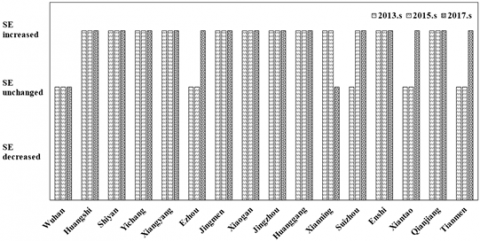
The results of the production scale of industrial parks in various regions of Hubei measured by single-stage DEA and three-stage DEA were plotted as shown in Figures 2 and 3. For five regions Wuhan, Shiyan, Jingzhou, Suizhou and Tianmen, their efficiency results between 2013 to 2017 measured by single-stage DEA were the same with the results measured by three-stage DEA; after environment factor and random factor adjustment, the SE of Huangshi, Yichang, Xiangyang, Jingmen, Xiaogan, Huanggang, Xianning, Enshi, Xiantao and Qianjiang had improved; only Ezhou’s SE in 2013 had decreased; generally speaking, compared with single-stage DEA, in the results of three-stage DEA, about 68% of the regions’ SE had changed.
In terms of the mean efficiency values, in single-stage DEA, there’s SE>PTE>TE; after environment factor and random factor adjustment, in three-stage DEA, there’s PTE>SE>TE. The single-stage DEA concluded that the under-scale of industrial parks is an important factor affecting their output efficiency, however, after environment factor and random factor adjustment, it’s found that the under-use and under-developed technology is the main factor affecting the output efficiency of industrial parks. The regression results of slack variables were relatively significant, the environment variables do have an impact on production efficiency, which had also proved the correctness of three-stage DEA from another perspective.
In terms of the production scale of industrial parks, the growth rate of the proportion of sized enterprises in the industrial parks of most regions was 45.6% (calculated from the Hubei Statistical Yearbook), and the results of three-stage DEA showed that the SE of most industrial parks in Huangshi, Jingzhou and Xiaogan was decreasing year by year, indicating that increasing the scale of the parks had a limited effect on efficiency improvement; by further analyzing the government’s technology investment it’s found that, the growth rates of technology investment of Wuhan, Shiyan, Huangshi, Yichang, Xiaogan, Jingzhou, Huanggang, Xianning, Suizhou, Xiantao, Qianjiang and Jingmen all exceeded 100%, and the growth rate of authorized patents also exceeded 100%. The results of the three-stage DEA showed that the PTE of above regions had also increased year by year, indicating that improving production technology is the key to improving the output efficiency of industrial parks, which had also verified the correctness of three-stage DEA.
Figure 2. SE of industrial parks in Hubei province between 2013 and 2017 (single-stage DEA)
Figure 3. SE of industrial parks in Hubei province between 2013 and 2017 (three-stage DEA)
Aiming at the measurement of the efficiency of industrial parks, this paper adopted three-stage DEA within the framework of production function to measure the output efficiency of industrial parks in various regions of Hubei Province. The three-stage DEA can eliminate the influence of environment factors and random factors, and the research results showed that:
(1) Under the condition that the influence of non-production factors was not eliminated, only Wuhan, Yichang, Suizhou and Qianjiang were at the frontier of effective efficiency, and only half of the regions were in the stage of RTS increase, a few regions were in the stage of RTS decrease, and there’s SE>PTE>TE.
(2) After environment factors such as public facilities and services, social consumption level, tax policy degree of openness, regional industrial structure and technical innovation ability had been controlled, SFA function was applied to conduct regression analysis on the slack variables of the first-stage DEA, and the results showed that the influence of environment factors on slack variables was significant, indicating that environment factors have an impact on the efficiency of industrial parks.
(3) The efficiency analysis results obtained after the original input-output data had been adjusted according to the regression coefficients of SFA showed that, more than half of the industrial parks in Hubei Province were in the stage of RTS increase, and there’s PTE>SE>TE, which was consistent with the actual conditions of the industrial parks in Hubei Province.
The above research results suggested that, the low output efficiency of industrial parks was mainly due to the inefficiency caused by the backward technology. The SFA regression results showed that, public facilities and services, social consumption level, tax policy, degree of openness, regional industrial structure, and technical innovation ability all had a great impact on the output efficiency of industrial parks in Hubei province, therefore, this paper proposes that the local governments can make efforts to promote the output efficiency of industrial parks from the following 5 aspects: (1) Comprehensively promote the construction of public facilities of the cities in which the industrial parks are located, and offer necessary public services to provide a good guarantee for the production of industrial parks (measured by the proportion of basic infrastructure investment and public budget expenditures in the GDP); (2) Expand the regional consumer market and stimulate regional consumption potential (measured by the total retail sales of social consumption); (3) Increase tax incentives for technology companies in industrial parks, through tax incentives, risk compensation and other incentive policies, guide various guarantee agencies to actively provide guarantee services for the loans of technical innovation projects and independent intellectual property industrialization projects of small and medium sized companies (measured by the proportion of tax revenue of industrial parks in the GDP); (4) Actively introduce foreign capital and promote regional industrial transformation and upgrading (measured by the proportion of the primary and tertiary industries in the total output of the region); (5) Encourage financial institutions to actively support the technological innovation of small and medium-sized enterprises (measured by the number of patents of the region), cultivate high-tech industrial clusters, and promote the formation of high-tech industrial chain.
This paper was supported by ‘Research on the Effect of Regional Science and Technology Innovation of Small and Medium-sized Enterprises in Wuhan Urban Circle’, project of Hubei Small and Medium-sized Enterprises Research Center (project No.: HBSME2019C12) and ‘Study of <International Economics> Bilingual Education Re-form’, project of The Ministry of Education production-study-research cooperation (project No. :201901067019).
[1] Tone, K. (2001). A slacks-based measure of efficiency in data envelopment analysis. European Journal of Operational Research, 130(3): 498-509. https://doi.org/10.1016/S0377-2217(99)00407-5
[2] Oggioni, G., Riccardi, R., Toninelli, R. (2011). Eco-efficiency of the world cement industry: A data envelopment analysis. Energy Policy, 39(5): 2842-2854. https://doi.org/10.1016/j.enpol.2011.02.057
[3] Wu, Y., Zhang, X., Skitmore, M., Song, Y., Hui, E.C.M. (2014). Industrial land price and its impact on urban growth: A Chinese case study. Land Use Policy, 36: 199-209. https://doi.org/10.1016/j.landusepol.2013.08.015
[4] Demerjian, P.R. (2017). Calculating efficiency with financial accounting data: Data envelopment analysis for accounting researchers. SSRN Electronic Journal. https://doi.org/10.2139/ssrn.2995038
[5] Aldamak, A., Zolfaghari, S. (2017). Review of efficiency ranking methods in data envelopment analysis. Measurement, 106: 161-172. https://doi.org/10.1016/j.measurement.2017.04.028
[6] Fried, H.O., Lovell, C.A.K., Schmidt, S.S., Yaisawarng, S. (2002). Accounting for environmental effects and statistical noise in data envelopment analysis. Journal of Productivity Analysis, 17(1-2): 157-174. https://doi.org/10.1023/A:1013548723393
[7] Saati, S., Hatami-Marbini, A., Agrell, P.J., Tavana, M. (2013). A common set of weight approach using an ideal decision making unit in data envelopment analysis. Journal of Industrial & Management Optimization, 8(3): 623-637. https://doi.org/10.3934/jimo.2012.8.623
[8] Monika, D., Mariana, S. (2015). The using of data envelopment analysis in human resource controlling. Procedia Economics & Finance, 26: 468-475. https://doi.org/10.1016/S2212-5671(15)00875-8
[9] Benicio, J., de Mello, J.C.S. (2015). Productivity analysis and variable returns of scale: DEA efficiency frontier interpretation. Procedia Computer Science, 55: 341-349. https://doi.org/10.1016/j.procs.2015.07.059
[10] Chen, C., Lam, J.S.L. (2018). Sustainability and interactivity between cities and ports: A two-stage data envelopment analysis (DEA) approach. Maritime Policy and Management, 45(7-8): 944-961. https://doi.org/10.1080/03088839.2018.1450528
[11] Zhang, H., Song, W., Peng, X., Song, X. (2012). Evaluate the investment efficiency by using data envelopment analysis: The case of China. American Journal of Operations Research, 2(2): 19933. https://doi.org/10.4236/ajor.2012.22020
[12] Lamb, J.D., Tee, K.H. (2012). Data envelopment analysis (DEA) integrated risk assessment technique on hedge funds investment: theory and practical application. SSRN Electronic Journal. https://doi.org/10.2139/ssrn.2005820
[13] Cook, W.D., Imanirad, R. (2011). Data envelopment analysis in the presence of partial input-to-output impacts. Journal of CENTRUM Cathedra: The Business and Economics Research Journal, 4(2): 182-196. https://doi.org/10.7835/jcc-berj-2011-0057
[14] Johnes, J. (2006). Data envelopment analysis and its application to the measurement of efficiency in higher education. Economics of Education Review, 25(3): 273-288. https://doi.org/10.1016/j.econedurev.2005.02.005
[15] Bosetti, V., Locatelli, G. (2006). A data envelopment analysis approach to the assessment of natural parks' economic efficiency and sustainability. The case of Italian national parks. Sustainable Development, 14(4): 277-286. https://doi.org/10.2139/ssrn.718621
[16] Camanho, A.S., Dyson, R.G. (2006). Data envelopment analysis and Malmquist indices for measuring group performance. Journal of Productivity Analysis, 26(1): 35-49. https://doi.org/10.1007/s11123-006-0004-8
[17] Kuosmanen, T., Kortelainen, M. (2005). Measuring eco-efficiency of production with data envelopment analysis. Journal of Industrial Ecology, 9(4): 59-72. https://doi.org/10.1162/108819805775247846
[18] Bosetti, V., Cassinelli, M., Lanza, A. (0). Using data envelopment analysis to evaluate environmentally conscious tourism management. SSRN Electronic Journal. https://doi.org/10.2139/ssrn.541124
[19] Johnes, J. (2006). Measuring efficiency: A comparison of multilevel modelling and data envelopment analysis in the context of higher education. Bulletin of Economic Research, 58(2): 75-104. https://doi.org/10.1111/j.0307-3378.2006.00238.x
[20] Morita, H. (2003). Analysis of economies of scope by data envelopment analysis: Comparison of efficient frontiers. International Transactions in Operational Research, 10(4): 393-402. https://doi.org/10.1111/1475-3995.00415
[21] Goto, J.N. (2003). Measurement of dynamic efficiency in production: An application of data envelopment analysis to Japanese electric utilities. Journal of Productivity Analysis, 19(2-3): 191-210. https://doi.org/10.1023/A:1022805500570
[22] Simar, L., Wilson, P.W. (2007). Estimation and inference in two-stage, semi-parametric models of production processes. Journal of Econometrics, 136(1): 31-64. https://doi.org/10.1016/j.jeconom.2005.07.009
[23] Bloom, D.E., Canning, D., Sevilla, J. (2004). The effect of health on economic growth: A production function approach. World Development, 32(1): 1-13. https://doi.org/10.1016/j.worlddev.2003.07.002