Agus Hermanto![]() | Diki I. Permana*
| Diki I. Permana*![]() | Dani Rusirawan
| Dani Rusirawan![]() | Tito Shantika
| Tito Shantika![]()
© 2023 IIETA. This article is published by IIETA and is licensed under the CC BY 4.0 license (http://creativecommons.org/licenses/by/4.0/).
OPEN ACCESS
The energy potential of low-head water can be exploited by using the horizontal axial flow to produce rotation in the turbine, which is then converts it into electricity in the generator. The types of blades that are commonly used are propeller types, cross-flow types, and Kaplan types. In this research, a prototype of micro-hydro power plant with a capacity of 20 W will be developed, which utilizes the potential of water flow with a head < 0.5 m. This research begins with observing water flow, including flow characteristics and parameters such as speed, head, and available discharge. The next step is to design the power plant, which includes the design of a very low head horizontal axial turbine, turbine structure and accessories, turbine blade rotor, power transmission system, generator selection, and control system. The manufacture of the main components of the turbine, reservoir, diffuser, etc., is carried out before integrating the entire micro hydropower system. The result shows the physical model of the very low-head turbine prototype produces power at the highest Head (0.4 m) of 11.02 W, while at the same Head, the computational fluid dynamic (CFD) results produce the most significant power with 13.55 W.
hydro turbine, micro-hydro, power generation, Kaplan turbine, cross-flow turbine, very low head
Electricity is one of the essential infrastructures to support the economic growth of a country. The projected growth of electricity demand in Indonesia using the assumption of economic growth for ten years with an average of 6.2% per year and moving from the realization of electricity demand in 2009 is estimated to reach 334.4 TWh or an average growth of 9.3% in 2019 [1]. Meanwhile, the national electricity production in Indonesia until November 2015 was 283 TWh, with the national electrical energy consumption reaching 228 TWh. The total installed capacity in Indonesia of 54,488 MW, 70% or 38,204 MW is owned by Electrical State Company (ESC) (PT. PLN), followed by Independent Power Producer (IPP) as much as 21% or 11,519 MW, and the rest by Private Production Utility (PPU) and Operating Permit (OP) non-fuel as much as 9% or 4,765 MW [2]. Half of the total electricity generated is produced by coal-fired power plants. Furthermore, the national electrification ratio was recorded at 88.3% in each province. Several regions in Indonesia still have electrification ratios below 70%, including Central Kalimantan, East Nusa Tenggara, North Sulawesi, and Papua. To support national economic growth and equitable development, the Indonesian government has set a national electrification target of 99.7%, which must be achieved by 2025 [2]. To achieve this target, electrical energy must be distributed to all regions in Indonesia, remote rural areas, isolated systems, and small islands.
In rural areas in Indonesia, available water sources such as springs, rivers, agricultural irrigation canals, and others can be used as power plants. Irrigation channels generally do not have a significant head difference, but there is a large enough flow of water to have a large enough water energy potential. Therefore, the two parameters, namely the water supply pressure, which represents the head (waterfall), and the water flow rate, are essential to be determined earlier in order to estimate the potential output power [3]. This is a challenge for researchers to realize a micro-hydro power plant with a capacity of 20 kW with a low head. The generator assumes that one house consumes 200 Watts of power so that it can illuminate about 100 houses around the irrigation canal. The amount of electrical energy generated from this power plant is sufficient with the assumption that electrical energy is used for irrigation pumps during the day and lighting at night.
Micro-hydro turbine research should ideally be conducted on the prototype itself. However, such studies are difficult due to the vast sizes needed as well as the expenses, mostly due to production losses. In the literature, only a few research on full-scale turbines are known [4, 5]. Sutikno and Adam [6], conduct a numerical simulation and experimental of the very low head turbine under 1.2 meter and the minimal pressure coefficient and free vortex criteria for axial-flow hydraulic turbines are presented. While Borkowski et al. [7], examines a small hydropower facility that operates at variable speed. The hydro-set, which comprises guiding vanes and a propeller turbine coupled with a permanent magnet synchronous generator, is modeled using CFD, and the experimental results are compared. None of these provide the same degree of information as trials conducted on models where optical techniques may be utilized to assess velocity. Full-scale measurements are often restricted to pressure and strain measurements in the stationary domain [8, 9]. Taking measurements on a runner [10, 11] adds another level of complexity that has only been seen in a few studies.
Detail modeling is necessary to support the design process and identify the operating conditions of the integrated turbine with the wet gap. The CFD approach is the most appropriate when considering qualitative and quantitative findings and fluid flow device analysis with complicated geometries [12-14]. So far, several CFD simulations of water turbines have been performed. Božić and Benišek [15] computed total secondary losses in the Kaplan turbine runner by integrating computational findings from two turbulence models (blade SST and SGG models) and experimental data on profile features. Javadi and Nilsson [16] used RNG K-epsilon (a conventional eddy-viscosity model), explicit algebraic Reynold stress model (EARSM) and SSTCC (non-conventional eddy-viscosity models), and DDES-SA to simulate the U9 Kaplan turbine model. Gohil and Saini [17] investigated the Francis turbine and used the SST (Shear Stress Transport) turbulence model and two-phase cavitation flow model to simulate unsteady (transient) viscous flow. The analysis is based on the homogeneous mixture method, with a Rayleigh Plesset equation solved using the ANSYS CFX code.
Although CFD analysis has been carried out to predict how much power and efficiency the Kaplan turbine will produce. However, the manufacturing and analysis results of the Kaplan turbine prototype will significantly impact the optimal design and characteristics of the Kaplan turbine located in the actual rural area [18].
From the literature above regarding the design, manufacture, and testing of low-head turbines, a small-scale prototype model is needed to determine the prototype turbine's driven characteristics that will be applied to the original size turbine. Therefore, this research aims to design and build a prototype micro hydro power plant with a capacity of 20 Watts using a shallow head horizontal axial turbine by utilizing the flow of irrigation channels in rural areas and to determine the performance and characteristics of the power plant.
2.1 Design of Kaplan turbine
Hydroelectric Power Plants are distinguished according to the capacity of the generated electricity generation. The magnitude of the available hydropower potential occurs when the water source experiences a flow of water falling from a high level to a low level vertically (H), this parameter is crucial in the generation of hydroelectric energy. In contrast, water that flows (Q) very quickly does not contain enough energy for producing electrical energy except in the case of hydroelectric power. On a huge scale, these two parameters, namely the fall of water and the flow of water available in one source, will produce quite a large amount of energy.
The available energy potential for electricity generation can be calculated based on the Eq. (1) [19]:
$P=\rho . g . Q . H . \eta$ (1)
$\eta=\frac{\text { Output Power }}{\text { Input Power }} \times 100$ (2)
where, P: power (watt), ρ: water density (1000 kg/m3), g: the acceleration of gravity constant (9.81 m/s2), Q: flow rate (m3/s), H: Head net (m), η: efficiency system (%).
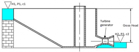
The power produced by the generator can be obtained by multiplying the efficiency of the turbine (η) and generator with the theoretical power. As can be understood from the formula above (Eqns. (1)-(2)), the power generated is the product of the height of the fall or the head net (H) and the large water discharge effectively (Q) and economically [20]. Figure 1 shows the schematic of a micro hydro power plant. In this study, the proposed power of micro-hydro model is around 20 W with the height of the source is shallow, which is less than 50 cm. From the value of the water flow and head, it can be identified the type of turbine will be used based on the turbine operating regime and then the appropriate type of flow is the type of axial flow with a Kaplan-type turbine [21].
After that, determine the specific speed that related with power (P) and head (H) shown by Eq. (3) with maximum value (Eq. (4)) and minimum value (Eq. (5)). The specific speed is an essential parameter in designing a turbine that is used in a generating system, including determining the type of turbine to be used, determining the rotational speed of the turbine during operation, and determining the geometry of the turbine, especially the dimensions of the tip diameter and hub diameter.
$N s=n \sqrt{\frac{P}{H^{5 / 4}}}$ (3)
$N_{s_{-}} \max =\frac{2702}{\sqrt{h}}$ (4)
$N_{s \_} \min =\frac{2088}{\sqrt{h}}$ (5)
where, n: the turbine speed (rpm), ns: the specific speed, P: Output Turbine (kW), H: head (m). Limitation of the specific speed value based on the reference from ESHA is 0.19≤Ns≤1.55 [22], and based on the reference from JICA, 250≤Ns≤1000 [23]. The equation used to get the maximum specific speed value based on JICA is as follows:
$N_s-\max \leq(20000 /(H+20))+5$ (6)
Figure 1. The schematic of micro-hydro power
In hydropower plants using an axial flow turbine propeller, the average running speed of the runner operates at a rotational speed below 1000 rpm, thus the calculation to find the appropriate runner dimensions that can be applied using various runner speeds of 300, 500, 700, and 900 rpm. The rotating speed varies so that it can determine the characteristics of the runner's dimensions. While the runner diameter (De) and hub diameter (Di) are shown by Eqns. (7) and (8). While Nqe is specific speed according to flow magnitude (Eq. (9)) [21].
$D_e=84.5 \times\left[0.79+\left(1.602 \times N_{q e}\right)\right] \times \frac{\sqrt{H_n}}{60 \times n}$ (7)
$D_i=\left(0.25+\frac{0.0951}{N_{q e}}\right) \times D_e$ (8)
$n_{Q E}=\frac{n \sqrt{Q}}{E^{3 / 4}}$ (9)
The suction head is the height of the center line runner to the downstream water level. The turbine is above the water level if the suction head is positive. The negative value is when the turbine below the waterline. To avoid cavitation, the suction head range is limited. The maximum allowable suction head can be calculated using the following Eq. (10). Modeling tests calculate the cavitation coefficient (σ), usually supplied by the turbine manufacturer. However, statistical studies related the cavitation coefficient to specific velocities. So the cavitation coefficient for the Kaplan turbine can also be made by the following Eq. (11). However, in this study, a small-scale model with a capacity of 20 Watts will be made, so it can be assumed that cavitation calculations are negligible.
$H s=\frac{P_{a t m}-P_v}{\rho x g}+\frac{C_4^2}{2 g}+\sigma \times H n$ (10)
$\sigma=1.5241 \times N_{Q E}^{1.46} \times \frac{C_4^2}{2 \times g \times H n}$ (11)
2.2 The blade design of Kaplan turbine
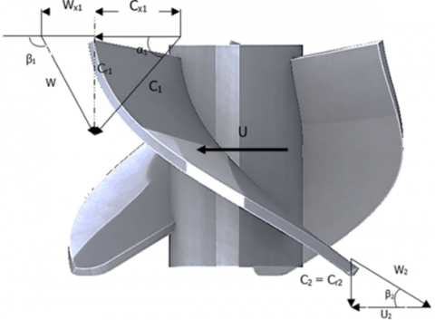
The turbine blade design is based on the velocity triangle diagram for an axial flow turbine, as shown in Figure 2, and using the equations below, the equations used are as follows in Table 1. The mean radius generally represents the velocity triangle. The flow velocity is axial at the inlet and outlet so that Cr1=Cr2=Ca. The blade velocity vector U1 is obtained from the absolute velocity vector C1 (at an angle β1 to U1) to produce the relative velocity vector W1. For maximum efficiency, the vortex component Cx2=0, where the absolute speed of the turbine blade output is axial. So C2=Cr2 [21].
Table 1. The equations of blade design
|
Description |
Equations |
No of equation |
|
Tangential velocity component |
$U=\frac{\pi \cdot n \cdot D}{60}$ |
(12) |
|
$C X_1=\frac{H_{\text {static }} \; \cdot \, g}{U}$ |
(13) |
|
|
$w X_1=U-C X_1$ |
(14) |
|
|
Axial velocity component |
$C_a=\frac{Q \times 4}{\pi \times \left(D_e^2-D_i^2\right)}$ |
(15) |
|
Inlet angle |
$\tan \left(180^{\circ}-\beta_1\right)=\frac{C_a}{w X_1}$ |
(16) |
|
Outlet angle |
$\tan \beta_2=\frac{C_a}{U}$ |
(17) |
|
Mean diameter |
$d_m=\frac{D_e+D_i}{2}$ |
(18) |
The number of propeller turbine blades is generally four to six, in this plan the number of blades used is four blades, so the number is taken because generally the maximum limit for use is 12 m head [21]. However, in determining chord and pitch is based on the comparison value between pitch and chord with a comparison value of 1-1.5. The chord is the length from the leading edge to the tailing edge of the turbine blade, and pitch is the distance between chords; the comparison equation is as follows [21]:
$\sigma=\frac{S}{C}$ (19)
$S=\frac{2 \pi r}{Z}$ (20)
Figure 2. The velocity triangle of blade turbine
where, β is angle of blade (°), C is absolute velocity (m/s), Cr is axial velocity (m/s), W is relative velocity (m/s), α is absolute angle (°), U is blade velocity (m/s), and subscript 1 and 2 representing of inlet and outlet blade, respectively.
Meanwhile, σ is the comparison value, S is pitch (m), C is chord and Z is the number of blade. In designing the dimensions of the turbine runner blades, the average (mean) diameter will be studied. In this section, the final result will be the type of profile (airfoil) that must be used. Here are some calculations to get the type of profile used:
The lift coefficient:
$\zeta_a=\frac{{w_2}^2-w_{\infty}^2+2 g \times \left(P_{a t m}-H_s-P_{\min }-\eta_s \frac{C_3{ }^2-C_4^2}{2 g}\right)}{K \times W_{\infty}{ }^2}$ (21)
$\frac{l}{t}=\frac{g \times H_n}{W_{\infty}^2} \times \frac{C_a}{U} \times \frac{\cos \lambda}{\sin 180-\beta_1-\lambda} \times \frac{1}{\zeta_a}$ (22)
$\zeta_A=\frac{\zeta_a}{\zeta_a / \zeta_A}$ (23)
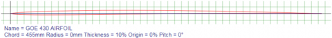
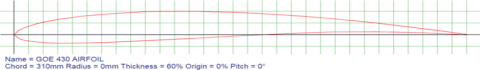
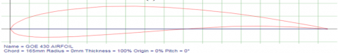
In order to reduce the drag force with using Eqns. (19)-(20), a study was carried out on the mean diameter, and the lift coefficient value ζA=0.525 was obtained. With the value of the lift coefficient obtained, the Gottingen 430 airfoil was chosen because it has a drag coefficient value of ζW=0.0088, which is smaller than the Gottingen 432 with a drag coefficient of 0.010. Figure 3 shows the profile of Gottingen 430 airfoil using airfoiltools.com.
(a) Tip diameter
(b) Mean diameter
(c) Hub diameter
Figure 3. Airfoil profile
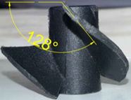
(a) Model view
(b) Inlet angle view
(c) Outlet angle view
Figure 4. Turbine prototype geometry
Table 2. The parameter design and experimental
|
Parameters |
Value |
Units |
|
Wtarget |
20 |
W |
|
ηgenerator |
75 |
% |
|
ηturbine |
90 |
% |
|
Hnett |
0.5 |
m |
|
Q |
1.35 |
m3/s |
|
N |
240 |
rpm |
|
Ns |
4.21 |
- |
|
De |
48 |
mm |
|
Di |
23 |
mm |
|
Dhub |
10 |
mm |
|
β1 |
128 |
o |
|
β2 |
31 |
o |
After getting all the main parameters needed to design the turbine, as shown in the Table 2, the calculation results from the turbine speed triangle are obtained so that the shape of the turbine according to the design can be formed and shown in the Figure 4. Physical modeling uses turbine blades with a diameter of 48 mm and a maximum head of 50 cm. This modeling aims to obtain information that the designed system can work properly and produce turbine shaft rotation. In this physical modeling, the turbine is coupled with a DC generator with a capacity of 20 Watt, and the electric load uses 3 of 5 Watt lamps each.
2.3 Experimental setup
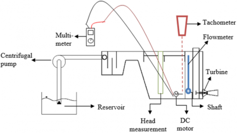
Figure 5 is the model testing scheme carried out at several variations of water levels to obtain values from the parameters of the turbine system with two methods (the centerline model is above tail race water surface and below tail race water surface), turbine rotation speed, and the flow discharge that occurs. To finding the water level in the model, a measurement of the water level is carried out using a ruler which will be attached to one of the side walls of the model so that it can be easily seen how high the water level is. This turbine system model is a turbine that can rotate with a very low head. The method used is to use a tachometer measuring device from The Fluke 930 (accuracy ± 0.02% ± 2 dgt) which will be directed from the top of the model to the disc connected to the turbine shaft so that later it will get the turbine's rotational speed at a predetermined water level. The outflow water is obtained by flow-meter from Flowatch FL-03 that enters the turbine, and then it will be multiplied by the area of the turbine input area so that it will be known how much discharge is flowing. The next step is to measure the voltage and current using a multi-meter from Hioki 3801-50 attached (accuracy ± 0.025% rdg. ± 5 dgt) to the DC motor.
Figure 5. The schematic of experimental setup
The CFD model was created in ANSYS R17. The integrated computer engineering and manufacturing (ICEM) utility is used to construct the grids, and the ANSYS CFX code is used to execute the transient simulations. A second-order accurate finite-volume discretization approach is used to solve the incompressible RANS equations. To represent the turbulence components of the RANS equations, the shear stress transport (SST) k-ω turbulence model is chosen due to its accuracy, as shown by Menter [24]. The k- turbulent model is appropriate for simulating turbulence in areas far from the wall but not near walls or at low Reynolds Numbers. The k-turbulent model is the inverse of this. As a result, in the turbulent k- SST model, the blending function serves as a switching function. Turbulence will be represented using k-ω, while in the boundary layer region (near the wall), and with k-Ɛ when outside the boundary layer (free stream).
At this simulation stage, the turbine system is divided into six parts, namely: reservoir 1, reservoir 2, reservoir 3, reservoir 4, rotor blade, and diffusers; the turbine system is divided into six parts so that it is easy to determine the mesh to be given as shown by Figure 6. The 3D image input into the pre-processor stage is the part of the system that will be flowed by the working fluid. Because the CFX simulation applies to the part that is flowed by the fluid must be in solid form. In contrast, if there is a wall inside the system, then it must be used as the space shown in Figure 7a. There are parameters at the meshing stage to see whether the meshing quality is good. Namely, by bringing up options in statistics and then selecting mesh metrics, several options will appear. The options used include skewness. In the skewness option, if the mesh value is close to 0 (zero), then the quality of the mesh is excellent (Figure 7b), but if it is close to 1 (one), then the quality of the mesh is poor. Table 3 displays the reservoir 1 and 2, reservoir 2 and 3, runner, and diffuser's detailed mesh number, skewness, and orthogonal quality. The average skewness values of the reservoir 1 and 2, reservoir 2 and 3, and diffuser are 0.22, 0.24, and 0.20, respectively, in Table 3. Reservoir 1 and 2, reservoir 2 and 3, and diffuser have orthogonal values of 0.88, 0.87, and 0.88, respectively. Table 4 summarizes the pre-processing method for defining boundary conditions and settings relating to other simulation input parameters.
Figure 6. Turbine model components
Figure 7. Turbine geometry: a) turbine 3D, b) mesh profile
Table 3. Detailed mesh of the turbine
|
Component |
Grid Number |
Evaluation Criteria |
Value |
|
Reservoir 1 & 2 |
1,162,734 |
Max skewness Avg skewness Min orthogonal Avg orthogonal |
0.97 0.22 0.09 0.88 |
|
Reservoir 3 & 4 |
1,400,740 |
Max skewness Avg skewness Min orthogonal Avg orthogonal |
0.86 0.24 0.20 0.87 |
|
Turbine |
976,528 |
Min Face Angle (o) Max Face Angle (o) Min Volume (m3) Max Edge Length Ratio |
18.5702 161.43 1.41x10⁻¹⁶ 242.537 |
|
Diffuser |
942,881 |
Max skewness Avg skewness Min orthogonal Avg orthogonal |
0.83 0.20 0.18 0.88 |
Table 4. The parameter input for simulation
|
Machine Type |
Axial Turbine |
|
Analysis Type |
Steady state |
|
Fluid |
H20 |
|
Reference Pressure |
0 (atm) |
|
Heat Transfer |
- |
|
Turbulence |
k-ω SST |
|
Inflow/Outflow Boundary Template |
Mass Flow Inlet P-static Outlet |
|
Inflow > T-Total |
23 (℃) |
|
Inflow > Volumetric flow rate |
Per Machine |
|
Inflow > Volumetric flow rate |
0.00377, 0.00455, 0.00494, 0.00572 (m3/s) |
|
Inflow > Flow Direction |
Normal to Boundary |
|
Outflow > P-static |
1 Bar |
|
Interface |
Frozen Rotor |
|
Solver Parameters > Advection Scheme |
High Resolution |
|
Solver Parameters > Convergence Control |
Physical Timescale |
This chapter will discuss the simulation results of the hydro turbine very low head performance both simulation and prototype experimental under the rotation range of 350 – 1300 rpm and Head variation from 0.1 – 0.4 m. Moreover, the analysis of flow characteristics such as velocity contour, velocity blade to blade, and streamline will be described.
4.1 Performance result
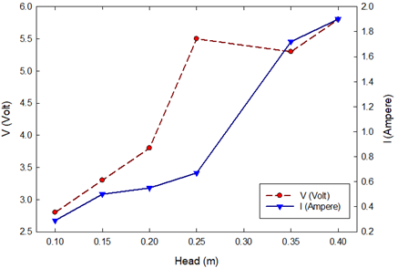
Figure 8 is an experimental result of a very low-head turbine prototype with an increase in the Head of the resulting voltage and electric current. We can see that the voltage results, the greater the Head, the greater the voltage generated, but there is a voltage drop of 0.2V at 0.35 m head, and it rises again up to 0.45 m with a voltage of 5.8V. The difference in the test location on the turbine centerline causes it. Where from a height of 0.1 - 0.25 m, the turbine centerline is below the tail race water level. While from a height of 0.3 - 0.4 m, the centerline of the turbine is above the water level of the tail race. The same result is shown by the current generated by the experiment, where a sharp increase of 1.05 A occurs from Head 0.25 m to 0.35 m. At that Head, the turbine rotation received is considerable (917 rpm), so the resulting increase in current is very significant.
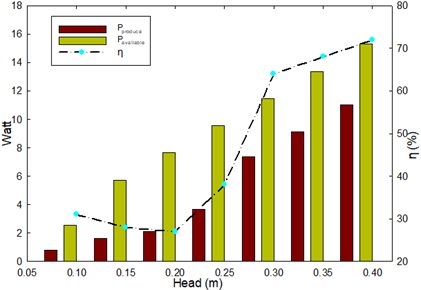
Figure 9 compares the generated power with the available power to the increase in Head (m). We can see that for every 0.1 m increase in Head, both Pproduce and Pavailable have increased, and at their peak, they produce the most significant power of 11.02 and 15.3 Watts at 0.4m, respectively. The similar results are shown by the efficiency produced as the head increases. In the range Head between 0.1 – 0.2 m, the efficiency decreases (4%); after that, it increases significantly, and the most significant value (72%) is at 0.4 m head. This is because the higher the Head, the greater the potential energy that the turbine will convert into kinetic energy. However, at heads below 0.2 m, not all available energy can be converted into turbine kinetic energy, causing small of Pproduce due to losses and causing efficiency to decrease. Another factor is the difference in test locations on the turbine centerline. Where from a height of 0.1 - 0.25 m, the turbine centerline is below the tail race water level. While from a height of 0.3 - 0.4 m, the centerline of the turbine is above the water level of the tail race.
Figure 8. Experimental result of H vs V and I
Figure 9. Experimental result of head vs Pproduce vs Pavailable and head vs ηoverall
Figure 10. Head vs Pexperiment and head vs Psimulation
The comparison graph of the power produced by the experimental and the simulation is shown in Figure 10. Whereas the head increases every 0.05 m, the amount of power produced, both experimental and simulated, increases. In more detail, there is a significant difference between the two types of power generated. This is very reasonable in that in the simulation, the losses that occur in the experiment are ignored, such as flow losses, friction losses, and other losses. Furthermore, the most significant power is generated at the highest head (0.4 m), whether an experiment or a simulation, with a magnitude of 11.02 and 13.55 kW, respectively.
4.2 Flow analysis
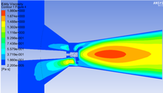
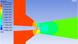
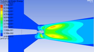
Figure 11 is a contour profile resulting from a low-profile turbine simulation at the highest head (0.4 m). Figure 11a shows the contour regarding the eddy viscosity. In the turbine inlet, the turbulent flow occurs in that section because the fluid density in that area is smaller, which is caused by a flow divergence of eddy viscosity value around 1.32 – 1.67 Pa.s. Meanwhile, in the diffuser (turbine outlet), the eddy viscosity value has increased significantly until it reaches 1.86, which means that the turbulence that occurs is considerable. It is because the flow velocity on the diffuser wall is very high due to the output from the nozzle. At the same time, there is much friction between the fluid driving on the diffuser side wall and the fluid in the diffuser center. The pressure contour shown in Figure 11b shows that the pressure in the reservoir is very high to the tip of the nozzle with a maximum value of 4.51 x 10³ Pa. While, at the nozzle outlet, the pressure decreases. It is due to the increase in the fluid velocity at the end of the nozzle after passing through the runner blades, and the fluid pressure is still low. The turbine outlet, which is the lowest fluid pressure at that point (3.867 Pa), is due to the very high fluid velocity. After the fluid enters the diffuser area, the pressure rises again because the velocity decreases. Figure 11c shows the contour of the turbulence kinetic energy caused by the high fluid velocity from the nozzle exit so that there is a shear stress between fluids with different velocities.
(a) Eddy viscosity
(b) Pressure
(c) Turbulence kinetic
Figure 11. Contour flow profile
(a) Upper view
(b) Side view
(c) Diffuser view
Figure 12. Streamline profile
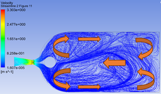
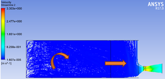
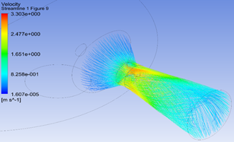
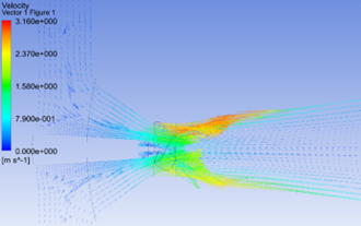
Figure 12 shows the flow pattern obtained from the simulation results. The flow pattern that occurs on the water surface from the end of the reservoir flows forward when at the reservoir edge with a semicircular cross-section, there is a backflow due to the flow from the reservoir inlet being turbulent that is shown by Figure 12a and 12b. In the streamlined direction, it can be seen that the fluid flow at the beginning of the reservoir rotates and then advances towards the right side. In Figure 12c, it can be seen on the outlet side. The middle of the diffuser zone looks empty. The centrifugal force causes this from the fluid flow momentum hitting the runner blades. So, the fluid moves following the diffuser’s wall. In the velocity vector shown in Figure 13, a whirlpool is caused by non-uniformity of the flow due to changes in cross-section. From the inlet to the nozzle outlet, the fluid flow pattern depicted is non-uniform. When it enters the runner inlet, the fluid velocity becomes faster due to the reduction in cross-section by the nozzle. The velocity decreases again when it passes through the diffuser, and the pressure increases.
Figure 13. Velocity vector
The design and experimental of the hydro-turbine very low head prototype was developed for initial research electricity generations in rural and remote area. The physical model of the very low-head turbine prototype produces power at the highest Head (0.4 m) of 11.02 W, while at the same Head, the CFD results produce the most significant power with 13.55 W. In the experimental, many losses occur that are not accommodated by CFD. The results of both CFD and experimental tests can provide a very significant initial step in designing, simulating, and conducting trials on an actual low very-head turbine which will be applied to a power of 20 kW. It can be note that the geometry of the nozzle and diffuser on the turbine draft tube greatly influences the momentum given by the water flow to the turbine blades. When the fluid passes through the runner, as much as possible, there should be no vortex because it can inhibit the rate of fluid that will come out after passing through the runner.
This research is funded with PUPT scheme of Ministry of Research, Technology and Higher Education Indonesia for community service in 2017.
|
C |
Axial velocity |
|
dm |
Mean diameter |
|
De |
Diameter runner |
|
Di |
Diameter hub |
|
g |
Acceleration of gravity constant, 9.81 m/s2 |
|
H |
Head, m |
|
N |
Rotational speed (rpm) |
|
Nqe |
Specific speed according flow magnitude |
|
Ns |
Specific speed |
|
Q |
Flow, (m3/s) |
|
P |
Power (W) |
|
S |
Pitch |
|
U |
Vector velocity |
|
w |
Relative velocity |
|
Z |
Number blade |
|
Abreviations |
|
|
ANSYS |
Analysis System |
|
CFD |
Computational Fluid Dynamic |
|
DC |
Direct Current |
|
EARSM |
Explicit Algebraic Reynold Stress Model |
|
ESC |
Electrical State Company |
|
ESHA |
European Small Hydropower Association |
|
JICA |
Japan International Cooperation Agency |
|
ICEM |
Integrated Computer Engineering and Manufacturing |
|
IPP |
Independent Power Producer |
|
PO |
Opertaing Permit |
|
PPU |
Private Production Utility |
|
RANS |
Reynolds-average Navier-Stokes |
|
RUPTL |
Rencana Usaha Penyediaan Tenaga Listrik |
|
SSG |
Speziale, Sarkar and Gatski |
|
SST |
Shear Stress Transport |
|
Greek symbols |
|
|
$\alpha$ |
Absolute angle, ° |
|
$\beta$ |
Blade angle, ° |
|
$\rho$ |
Density, kg/m3 |
|
$\sigma$ |
Cavitation coefficient |
|
$\eta$ |
efficiency, % |
|
$\zeta$ |
The lift coefficient |
|
Subscripts |
|
|
1 |
Inlet |
|
2 |
outlet |
|
net |
netto |
[1] PT. PLN. RENCANA USAHA PENYEDIAAN TENAGA LISTRIK (RUPTL). In: Direktorat Jenderal Ketenagalistrikan - Official Website. https://gatrik.esdm.go.id/, accessed on 5 Feb 2023.
[2] Kementrian Energi dan Sumber Daya Mineral International Coal Based Power Conferences 2016: Indonesia electricity In: Indonesia Electricity Development Plan annd Indonesia Coal-Ash Management Implementation. http://cdn.cseindia.org/userfiles/ilham.pdf, accessed on 5 Feb 2023.
[3] Shantika, T., Hartawan, L., Putra, M.A., Kurdi, A. (2018). Permanent magnet generator design and testing for hybride PV-picohydro. International Journal of Mechanical Engineering and Technology, 9(11).
[4] Unterluggauer, J., Sulzgruber, V., Doujak, E., Bauer, C. (2020). Experimental and numerical study of a prototype Francis turbine startup. Renewable Energy, 157: 1212-1221. https://doi.org/10.1016/j.renene.2020.04.156
[5] Trivedi, C., Gogstad, P.J., Dahlhaug, O.G. (2017). Investigation of the unsteady pressure pulsations in the prototype Francis turbines during load variation and startup. Journal of Renewable and Sustainable Energy, 9: 064502. https://doi.org/10.1063/1.4994884
[6] Sutikno, P., Adam, I.K. (2011). Design, simulation and experimental of the very low head turbine with minimum pressure and free vortex criterions. International Journal of Mechanical & Mechatronics Engineering, 11(1): 9-16.
[7] Borkowski, D., Węgiel, M., Ocłoń, P., Węgiel, T. (2019). CFD model and experimental verification of water turbine integrated with electrical generator. Energy, 185: 875-883. https://doi.org/10.1016/j.energy.2019.07.091
[8] Wang, F.J., Li, X.Q., Yang, M., Zhu, Y.L. (2009). Experimental investigation of characteristic frequency in unsteady hydraulic behaviour of a large hydraulic turbine. Journal of Hydrodynamics, Ser. B, 21(1): 12-19. https://doi.org/10.1016/S1001-6058(08)60113-4
[9] Trivedi, C., Gogstad, P.J., Dahlhaug, O.G. (2018). Investigation of the unsteady pressure pulsations in the prototype francis turbines – Part 1: steady state operating conditions. Mechanical Systems and Signal Processing, 108: 188-202. https://doi.org/10.1016/j.ymssp.2018.02.007
[10] Gagnon, M., Jobidon, N., Lawrence, M., Larouche, D. (2014). Optimization of turbine startup: Some experimental results from a propeller runner. IOP Conference Series: Earth and Environmental Science, 22: 032022. https://doi.org/10.1088/1755-1315/22/3/032022
[11] Presas, A., Luo, Y., Wang, Z., Guo, B. (2019). Fatigue life estimation of Francis turbines based on experimental strain measurements: Review of the actual data and future trends. Renewable and Sustainable Energy Reviews, 102: 96-110. https://doi.org/10.1016/j.rser.2018.12.001
[12] Ferziger, J.H., Perić, M., Street, R.L. (2002). Computational Methods for Fluid Dynamics. Berlin: Springer. https://doi.org/10.1007/978-3-642-56026-2
[13] Permana, D.I., Sutikno, P. (2019). Numerical simulation of turboexpander on organic Rankine cycle with different working fluids. IOP Conference Series: Materials Science and Engineering, 694(1): 012014. https://doi.org/10.1088/1757-899x/694/1/012014
[14] Gunawan, G., Permana, D.I., Soetikno, P. (2023). Design and numerical simulation of radial inflow turbine of the Regenerative Brayton cycle using supercritical carbon dioxide. Results in Engineering, 17: 100931. https://doi.org/10.1016/j.rineng.2023.100931
[15] Božić, I., Benišek, M. (2016). An improved formula for determination of secondary energy losses in the runner of Kaplan Turbine. Renewable Energy, 94: 537-546. https://doi.org/10.1016/j.renene.2016.03.093
[16] Javadi, A., Nilsson, H. (2017). Detailed numerical investigation of a Kaplan turbine with rotor-stator interaction using turbulence-resolving simulations. International Journal of Heat and Fluid Flow, 63: 1-13. https://doi.org/10.1016/j.ijheatfluidflow.2016.11.010
[17] Gohil, P.P, Saini, R.P. (2015). Effect of temperature, suction head and flow velocity on cavitation in a Francis turbine of small hydro power plant. Energy, 93: 613-624. https://doi.org/10.1016/j.energy.2015.09.042
[18] Wu, Y., Liu, S., Dou, H.S., Wu, S., Chen, T. (2012). Numerical prediction and similarity study of pressure fluctuation in a prototype Kaplan turbine and the model turbine. Computers & Fluids, 56: 128-142. https://doi.org/10.1016/j.compfluid.2011.12.005
[19] Munson, B.R., Young, D.F., Okiishi, T.H. (2002). Fundamentals of Fluid Mechanics. John Wiley and Sons, New York.
[20] Simpson, R., Williams, A. (2011). Design of propeller turbines for Pico Hydro - reca-corp.com. In: Design of propeller turbines for pico hydro. http://reca-corp.com/files/57898415.pdf, accessed on 6 Feb 2023.
[21] Lewis, R. (1996). Turbomachinery Performance Analysis. Elsevier: Butterworth-Heinemann.
[22] ESHA. (2004). Guide on how to develop a small hydropower plant. https://www.canyonhydro.com/images/Part_1_ESHA_Guide_on_how_to_develop_a_small_hydropower_plant.pdf, accessed on 6 Feb 2023.
[23] PPA. (2020). Micro hydropower system design guidelines. https://www.ppa.org.fj/wp-content/uploads/2020/10/Micro-Hydropwer-System-Design-Guideline-V1-4.pdf, accessed on 6 Feb 2023
[24] Menter, F.R. (1994). Two-equation eddy-viscosity turbulence models for engineering applications. AIAA-Journal, 32(8): 1598-1605.