Ximei Shi
© 2022 IIETA. This article is published by IIETA and is licensed under the CC BY 4.0 license (http://creativecommons.org/licenses/by/4.0/).
OPEN ACCESS
The obvious characteristics of urban thermal environment and heat island effect have brought a series of negative effects on urban ecosystem structure and residents' health. Scholars at home and abroad have conducted basic researches on urban thermal environment, but there is a lack of researches on areas with rapid urbanization and many interference factors. There are few researches on measures or suggestions to improve urban thermal environment and heat island effect from the perspective of ecological sustainable development. To this end, this paper conducts a study on thermal environment effect of landscape ecological pattern and dynamic analysis of pattern evolution. This paper, based on the radiative transfer equation method, carries out back calculation and back analysis on the parameters of urban surface temperature to obtain the dynamic characteristics of urban thermal ecological landscape pattern. By combining the obtained urban surface temperature with the landscape index, this paper analyzes the internal change of urban surface thermal ecological landscape pattern. Through the spatial characteristics of the barycenter of urban thermal environment effect, the expansion and development trend of urban thermal environment effect is revealed. Then based on Moran'sI coefficient, the whole spatial correlation of urban thermal environment effect and the degree of spatial aggregation in local areas are analyzed. Finally, the corresponding experimental results and analytical results are given in combination with the experiments.
landscape ecological pattern, urban thermal environment effect, analysis of pattern evolution of thermal environment
Along with the development of urbanization, the popularization and use of impervious surfaces such as cement, asphalt, reinforced concrete and glass cause great changes in the urban landscape structure [1-6]. Different landscape types have different thermal radiation characteristics, which will lead to change in the spatial relationship between urban landscape pattern and thermal environment [7-10]. At the same time, population migration significantly increases the heat discharge capacity of cities, accelerating different urban thermal environmental effects [11-17]. The obvious characteristics of urban thermal environment and heat island effect have brought a series of negative effects on urban ecosystem structure and residents' health [18-22]. Therefore, the thermal environment effect of urban landscape ecological pattern and pattern evolution has become one of the focus issues concerned by all walks of life.
In literature [23], the spatial Lorenz curve and distribution index are used to evaluate the thermal environment changes during the urbanization of Beijing metropolitan area from 2001 to 2009. In addition, the effect of landscape composition and spatial allocation on thermal environment are studied by correlation analysis and piecewise linear regression. Urban heat island (UHI) is more significant in summer than in spring, autumn and winter. Literature [24] first disposes 40 MOD11A2 scenarios recorded from 2003 to 2011 and then adopts two new methods: landscape centroid evolution and spatial autocorrelation. The maximum difference normalization method is used to divide the urban area of Beijing is into five parts: green island, weak heat island, heat island, strong heat island and serious heat island. Urban ecological environment effect is produced in the process of urbanization. Urban thermal environment is a comprehensive reflection of the environmental effects of urban landscape ecosystem. Literature [25] adopts Landsat TM/ETM+data, Modis data and real-time meteorological data to study the effect of landscape change on urban thermal environment. Modis data and satellite channel meteorological data are used to verify the effectiveness of Landsat TM/ETM+Band6. The annual and seasonal changes of thermal environment are revealed. In literature [26], a case study is conducted in Changchun, Jilin Province, China to further analyze the spatial pattern of urban landscape and urban thermal field. In addition, the influence of landscape pattern on urban thermal environment is discussed. The results show that the surface temperature of different types of urban landscape is obviously different. The average surface temperature of water body is the lowest and that of the industrial land is the highest, followed by commercial land, transportation land and public land. Besides, green landscape is one of the important factors that affect the distribution of urban thermal field, but the green patch area is not the main factor that determines land surface temperature. The average temperature is positively correlated with shape index and the lowest temperature is positively correlated with shape coefficient, while the lowest temperature is negatively correlated with green shape index.
It can be seen by combining the existing research results that scholars at home and abroad have conducted basic researches on urban thermal environment, but there is a lack of researches on areas with rapid urbanization and many interference factors. There are few researches on measures or suggestions to improve urban thermal environment and heat island effect from the perspective of ecological sustainable development. Therefore, this paper studies the thermal environment effect of landscape ecological pattern and dynamic analysis of pattern evolution. Firstly, in Chapter 2, this paper, based on the radiative transfer equation method, carries out back calculation and back analysis on urban surface temperature to obtain the dynamic characteristics of urban thermal ecological landscape pattern. In Chapter 3, the obtained urban surface temperature is combined with landscape index to analyze the internal changes of urban surface thermal ecological landscape pattern. In Chapter 4, this paper reveals the expansion and development trend of urban thermal environment effect through the spatial characteristics of the barycenter of urban thermal environment effect. Then based on Moran'sI coefficient, the whole spatial correlation of urban thermal environment effect and the degree of spatial aggregation in local areas are analyzed. Finally, the corresponding experimental results and analytical results are given in combination with the experiments.
The urban surface thermal environment is composed of different surface thermal ecological landscape. This paper takes the urban surface thermal environment as a complex regional complex to decompose the surface temperature pixels of several different regions. Then based on the radiative transfer equation method, this paper carries out back calculation and back analysis on urban surface temperature to obtain the dynamic characteristics of urban thermal ecological landscape pattern.
The use of the radiative transfer equation method is not limited by the range of thermal infrared remote sensing, but some known parameters, such as atmospheric upward and downward radiance and land surface emissivity are needed for relevant calculations. Assuming that the normalized differential vegetation index (NDVI) is represented by ZB and the vegetation coverage is EC, the formula for calculating the land surface emissivity is as follows:
$\sigma=0.004 G_1+0.986$ (1)
$E C=\frac{\left(Z B-Z B_{I D}\right)}{\left(Z B_{H U}-Z B_{I D}\right)}$ (2)
Assuming that the heat radiation intensity received by the sensor is represented by Ky, and the gray value of the pixel in the thermal infrared band is represented by CM, the following formula is given to calculate the spectral radiosity of the corresponding sensor:
$K_y=H_{x i m} \times C M+Y_{i x r}$ (3)
Assuming that the black-body radiance is represented by Px, the thermal infrared radiance is represented by Kμ, and the atmospheric transmissivity in the thermal infrared band is represented by τ, the atmospheric upward radiance, atmospheric transmissivity and atmospheric downward radiance are expressed by K↑, σ and K↓ respectively, then the formula for calculating the black-body radiance is as follows:
$P_x=\frac{K_\mu-K_{\uparrow}-\tau(1-\sigma) K_{\downarrow}}{t \sigma}$ (4)
Assuming that the real surface temperature by back calculation is represented by KRP, the black-body radiance is represented by Px, and the calibration parameters of infrared band are represented by L1 and L2, the real surface temperature can be obtained by the following formula
$K R P=\frac{L_2}{\ln \left(L_1 / P_x+1\right)}$ (5)
To calculate the spectral radiosity of the sensor accurately, the atmospheric effect in the tropics must be eliminated first. It is assumed that the spectral radiation is represented by Kμ, the quantized and calibrated standard pixel value is represented by W*, the multiplicative re-scaling factor for a particular band in the metadata is represented by NK, the re-scaling factor added for a particular band in the metadata is represented by XK, the quantized and calibrated standard maximum pixel value is represented by Wmax*, the highest radiance corresponding to Wmax*(CM = 255) is represented by KMAXμ, and the lowest radiance corresponding to Wmax*(CM=0) is represented by KMINμ. The formula for calculating the spectral radiance of the sensor after correction is given as:
$K_\mu=\left[\left(K_{M A X}{ }^\mu-K_{M I N}{ }^\mu\right) / W_{\max }{ }^*\right] \times W^*+K_{M N}{ }^\mu$ (6)
$K_\mu=N_\mu \times W^*+X_K$ (7)
It is assumed that the earth's surface is a black body with uniform emissivity, the atmospheric top brightness temperature is represented by AW, the thermal conversion constant of a specific band is represented by L1 and L2, and the atmospheric top spectral radiosity is represented by Kμ. The conversion of the thermal infrared band from atmospheric top radiation to the sensor brightness temperature can be performed based on:
$A W=L_2 /\left[\ln \left(L_1 / K_\mu+1\right)\right]$ (8)
Considering the threshold of NDVI, this paper analyzes the emissivity of different surface thermal ecological landscape. Assuming that the surface emissivity is expressed by σ, the exposed ZB value in thermal image is expressed by ZBmin, and the ZB value covered by vegetation is expressed by ZBnax, the following formula for calculating the land surface emissivity after correction is given:
$\sigma=0.004 \times\left[\left(Z B-Z B_{\min }\right) /\left(Z B_{\max }-Z B_{\min }\right)\right]^2+0.986$ (9)
Based on the existing grading method of urban surface temperature, this paper divides the surface temperature into seven grades by density division method, namely low temperature, relatively low temperature, secondary medium temperature, medium temperature, relatively high temperature, high temperature and extra-high temperature in order. Before formal grading of temperature, the temperature obtained by back calculation is normalized by the following formula to avoid the influence of inconsistant thermal imaging time on the grading result of temperature. Assuming that the normalized temperature value of the i-th pixel is represented by Fi, the value of the i-th pixel is denoted by Pi, and the maximum and minimum value of the effective temperature in the scene are denoted by Pmax and Pmin, respectively, then:
$F_i=\frac{P_i-P_{\min }}{P_{\max }-P_{\min }}$ (10)
In order to analyze the internal changes of urban surface thermal ecological landscape pattern, this paper combines the obtained urban surface temperature with landscape index. The specific landscape indexes include degree of aggregation, maximum patch index, spreading degree index, Shannon's diversity index, landscape separation degree index and number of patches.
Based on the degree of aggregation, this paper characterizes the aggregation of urban thermal ecological landscape patches. It is assumed that the maximum proximity between patches of the same type is represented by LJ, then:
$L J=\left[\sum_{i=1}^m\left(\frac{h_{i i}}{h_{i i \max }}\right) \times T_i\right] \times 100$ (11)
This paper characterizes the degree of dominance of urban thermal ecological landscape based on the maximum patch index. It is assumed that the total area of the landscape is represented by X, the area of patch ij is represented by xij, and the percentage of the maximum patch area of a certain landscape type in the total area of the landscape is represented by ηBK, then:
$\eta_{B K}=\frac{\max _{j=1}^n\quad\left( x_{i j}\right)}{X}$ (12)
In this paper, based on the spreading degree index, the degree of aggregation or spreading trend of different patches in urban surface thermal ecological landscape is characterized. Assuming that the area proportion of the patch type i in the landscape is represented by Ti and the number of patches present in the landscape is represented by n, there is:
$D E M=1+\frac{\sum_{i=1}^m \sum_{j=1}^m T_{i j} \operatorname{In}\left(T_{i j}\right)}{2 \operatorname{In}(m)}$ (13)
Based on Shannon's diversity index, this paper characterizes the change in the proportion of patch types in urban surface thermal ecological landscape. Assuming that the area proportion of the patch type i in the landscape is represented by Ti, there is:
$R F C J=-\sum_{i=1}^m \operatorname{In} T_i$ (14)
Based on landscape separation index, this paper characterizes the fragmentation degree of urban surface thermal ecological landscape
$C J U=\left[1-\sum_{i=1}^m\left(\frac{x_i}{X}\right)\right]$ (15)
In this paper, based on the number of patches, the fragmentation degree of regional surface thermal ecological landscape pattern is characterized
$M T=M_i$ (16)
This paper adopts transfer matrix method to analyze the change in spatial structure of urban thermal ecological landscape. Assuming that the urban thermal ecological landscape at the beginning and the end of the study is represented by Rij and the number of grades of the thermal ecological landscape is represented by m, the following formula shows the concrete expression
$R_{i j}=\left[\begin{array}{cccc}R_{11} & R_{12} & & R_{1 m} \\ R_{21} & R_{22} & \cdots & R_{2 m} \\ & \vdots & \ddots & \vdots \\ R_{m 1} & R_{m 2} & \cdots & R_{m m}\end{array}\right]$ (17)
Thermal admittance is often used to characterize the thermal behavior of urban surface thermal environment evolution. Impervious materials such as cement, asphalt, reinforced concrete, and glass that make up urban areas generally store or release energy at a lower rate than soil in suburban areas and have a greater influence on urban thermal climate change. If the thermal admittance value of a city is high, the surface temperature of the city changes slowly, and if the thermal admittance value of the city is low, the surface temperature of the city changes rapidly, especially at sunsets and sunrises when the temperature is prone to change a lot. Assuming that the heat island distribution index is represented by RF, a certain spatial unit of a city is represented by i, the area of the high temperature zone in the spatial unit is represented by Xfi, the area of the spatial unit is represented by Xi, the total area of all high-temperature zones in a city is expressed by Xm, and the total area of a city is expressed by X. Based on the heat island distribution index, the contribution degree of different urban areas to the overall urban thermal environment is characterized in this paper
$R F=\left(X_{f i} X\right) /\left(X_i X_m\right)$ (18)
The expansion and development trend of urban thermal environment effect can be revealed by the spatial characteristics of the barycenter of urban thermal environment effect. If the barycenter of urban thermal environment effect is deviated, the spatial distribution of urban thermal environment is unbalanced. This paper uses the barycenter to describe the spatial pattern change of the region where the thermal environment effect occurs in the city. The movement direction and distance of the barycenter can characterize the trend of the thermal environment effect changing with time. It is assumed that the longitude and latitude coordinate values in the area where the thermal environment effect occurs in a certain year of a city are represented by (Ap, Bp) respectively, the longitude and latitude coordinate values of the geometric center of the i-th heat island patch in year p of a city are represented by (ap,i,bp,i), the area of the i-th urban heat island patch in year p is denoted by FI_DQp,,i, the migration rate of the barycenter from the beginning y to the end x of the study is denoted by Ux-y, the barycentric coordinate value at the end of the study is represented by (Ax,Bx), and the barycentric coordinate value at the beginning of the study is represented by (Ay,By). The following formulas are to calculate the barycentric coordinate and migration rate of urban thermal environment effect
$A_p=\sum_{i=1}^m\left(F I_{-} D Q_{p, i} \times a_{p, i}\right) / \sum_{i=1}^m F I_{-} D Q_{p, i}$ (19)
$B_p=\sum_{i=1}^m\left(F I_{-} D Q_{p, i} \times b_{p, i}\right) / \sum_{i=1}^m F I_{-} D Q_{p, i}$ (20)
$U_{x-y}=\sqrt{\left(A_x-A_y\right)^2+\left(B_x-B_y\right)^2} /(x-y)$ (21)
The spatial attribute variables related to urban thermal environment effect have a certain spatial autocorrelation in the adjacent positions of a city. This paper uses Moran'sI coefficient to evaluate this relationship. Assuming that the bivariate overall Moran index is ZSxn,m, the standardized values of the standard deviations of the spatial elements x and y for n attribute value and m attribute value are represented by Mxn and Myn, the variance of n attribute and m attribute are represented by εn and εm, the weight matrix of the spatial elements is Qx,y, and the number of objects participating in the analysis is represented by E, the following formula is to calculate the bivariate overall Moran'sI coefficient
$Z S_{n, m}^x=\left(M_n^x Q_{x, y} M_m^y\right) / E$ (22)
$M_n^x=\left(A_n^x-\overline{A_n}\right) / \varepsilon_n$ (23)
$M_m^y=\left(A_m^y-\overline{A_m}\right) / \varepsilon_m$ (24)
The overall Moran'sI coefficient is mainly used to analyze the overall spatial correlation of urban thermal environment effect while the local LISA index is adopted to analyze the degree of spatial aggregation of spatial attribute variables related to urban thermal environment effect in local areas. Assuming that the standardized values of the spatial units x and y for the standard deviations of n attribute value and m attribute value are represented by Mxn and Mym, the formula for calculating the bivariate local Moran'sI coefficient Kxn,m is as follows:
$K_{n, m}^x=M_n^x\left(\sum_{y=1}^k Q_{x, y}\right) M_m^y$ (25)
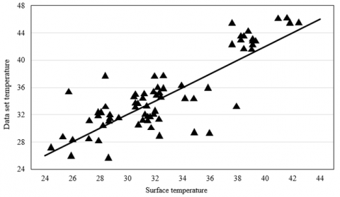
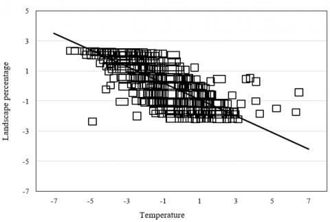
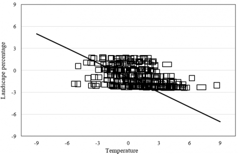
In order to analyze the inversion result, the discrete meteorological data are combined to verify the inversion based on the temperature data of the same day as the thermal imaging time. The spatial resolution of temperature data is 1,000m and that of thermal imaging data is 30m. The resolutions of the two kinds of data are different, so it is necessary to resample first. Then, 120 data points are randomly extracted from the two kinds of data for Pearson correlation analysis. Figure 1 shows the test result of urban thermal environment inversion accuracy. In this paper, the accuracy correlation coefficient of urban thermal environment inversion is more than 0.8, which meets the accuracy requirement.
Figure 1. Testing result of urban thermal environment inversion accuracy
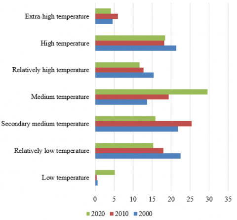
Figure 2. Statistical result of urban surface temperature
Figure 2 shows the statistical result of urban surface temperature in 2000, 2010 and 2020. It can be seen from the figure that from 1998 to 2018, the minimum surface temperature changed from 22.1℃ to 23.44℃, which was almost constant and kept at about 22℃, with a small variation range. The average surface temperature increased from 32.46℃ to 34.18℃, and the standard deviation decreased by 1.79℃. The average surface temperature of the target city increased year by year with the passage of time. However, there were differences among the thermal images in 2000, 2010 and 2020, so it is difficult to get the exact change characteristics of urban thermal landscape pattern and further study and analysis are needed.
Figure 3 shows the grades of urban surface temperature. It can be seen from the figure that in 2000, 2010 and 2020, relatively low temperature, secondary medium temperature and high temperature are temperature grades occupying a relatively high proportion in the urban area under study. As time goes on, the city develops continuously, the population grows rapidly, the impervious surfaces such as cement, asphalt, reinforced concrete and glass increase, and the temperature grade with higher proportion in the temperature area gradually becomes medium temperature area. At the same time, as the government vigorously promotes the policy of "returning farmland to forests", the forests in surrounding villages and towns of the city during the study increase, so the proportion of low-temperature urban areas also increases. By 2020, the proportion of low-temperature urban areas increased by 5.37%. Due to the low specific heat and strong thermal conductance of the earth's surface, the mountainous areas and bare areas of the city are concentrated in areas of relatively high temperature, high temperature and extra-high temperature. Compared with the surrounding green space, the thermal environment effect of the urban core area is more prominent, with a large range of heat island effect, so it is necessary to actively implement measures to improve the thermal environment effect.
Figure 3. Grades of urban surface temperature
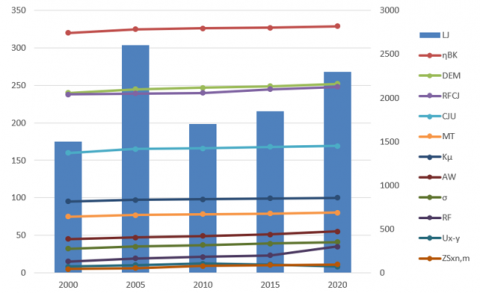
Figure 4. Change in urban thermal landscape pattern index
This paper analyzes the change of urban thermal landscape pattern index based on Fragstate software platform. Figure 4 and Table 1 show the interannual change of urban thermal landscape pattern index. During the period from 2000 to 2020, as urbanization accelerates, the urban spreading degree index increases slowly, the high-temperature patch concentration increases, and the landscape fragmentation becomes more and more obvious. The decrease in the degree of aggregation indicates that the degree of aggregation among the same type of urban patches decreases. The landscape shape index and Shannon's diversity index increase, indicating that the shape of urban patches is becoming more diversified and complicated. By comparing the landscape pattern change data of five years, we can see that the increase of landscape shape in medium temperature areas is small, and the change of landscape shape in secondary medium temperature areas is big. The main reason is that the urban built-up areas belong to medium temperature patch areas, and the dispersion degree of these areas is small. Natural vegetation and man-made green parks belong to secondary medium temperature patch areas, and the dispersion degree of these areas is large. The maximum patch index increases in different degrees in the medium and low temperature areas, and the degree of patch change is higher in the low and medium temperature areas.
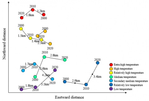
Figure 5. Evolution of barycenter of urban thermal grade
To deeply study the change of urban thermal landscape pattern, this paper constructs a centroid transfer analysis model of urban thermal environment effect areas, and calculates the barycenter of thermal patch areas corresponding to different thermal landscape, as well as analyzes the shift of urban surface thermal landscape during the study. Figure 5 shows the evolution of the barycenter of urban thermal grade. It can be seen from the figure that the shift of the barycenter of extra-high temperature landscape is weaker than that of low-temperature landscape. Due to the implementation of the government's "garden city" supporting greening programs, the thermal landscape ecological effect of urban part has been significantly improved and vegetation coverage has increased. With the increase of industrial mineral production in the surrounding areas, the extra-high temperature landscape areas transfer northwestward. The medium-temperature landscape areas, with the artificial parks as the center, shift eastward continuously, showing an obvious "continuous" expansion structure.
Correlation analysis result between the area percentage of different thermal landscape and thermal environment is shown in Figure 6. This paper adopts the bivariate overall Moran'sI spatial correlation analysis to divide the variable value into high area percentage and high temperature, high area percentage and low temperature, low area percentage and low temperature, low area percentage and high temperature, corresponding to the four quadrants in the two-dimensional plane coordinate. If the number of scattered points in quadrants 1 and 3 is larger than that in quadrants 2 and 4, it can be determined that there are fewer points where area percentage is inversely proportional to temperature, and the two variables are negatively correlated. As can be seen from Figure 6(1), the area percentage of urban thermal landscape has a strong negative correlation with temperature, which can reflect that when the area of natural vegetation, artificial green parks or water areas is large, the temperature will be lower. The above types of thermal landscape have a better mitigation effect on urban thermal environment. Figure 6(2) shows that the area percentage of urban landscape also has a strong negative correlation with temperature, which can reflect that forests or arable lands with high vegetation coverage also have a good mitigation effect on urban thermal environment.
Table 1. Interannual change of urban thermal landscape pattern index
|
Year |
LJ |
ηBK |
DEM |
RFCJ |
CJU |
MT |
|
2000 |
154.2 |
1.1783 |
47.4854 |
0.9932 |
92.3642 |
20.5283 |
|
2010 |
242.1 |
1.8612 |
46.2733 |
0.9869 |
90.9187 |
24.1885 |
|
2020 |
198.5 |
1.5289 |
44.9512 |
0.9871 |
90.7971 |
24.5156 |
|
Year |
Kμ |
AW |
σ |
RF |
Ux-y |
ZSxn,m |
|
2000 |
50.552 |
1.7349 |
4.4254 |
1.3465 |
5.774 |
3.675 |
|
2010 |
51.0931 |
1.7385 |
9.2357 |
1.3187 |
5.942 |
3.256 |
|
2020 |
55.0051 |
1.7862 |
9.2512 |
1.3739 |
6.234 |
3.047 |
(1)
(2)
Figure 6. Correlation analysis result between the area percentage of different thermal landscape and thermal environment
This paper conducts a study on thermal environment effect of landscape ecological pattern and dynamic analysis of pattern evolution. Based on the radiative transfer equation method, this paper carries out back calculation and back analysis on urban surface temperature to obtain the dynamic characteristics of urban thermal ecological landscape pattern. By combining the obtained urban surface temperature with the landscape index, this paper analyzes the internal change of urban surface thermal ecological landscape pattern. Through the spatial characteristics of the barycenter of urban thermal environment effect, the expansion and development trend of urban thermal environment effect is revealed. Then based on Moran'sI coefficient, the whole spatial correlation of urban thermal environment effect and the degree of spatial aggregation in local areas are analyzed. The test result of urban thermal environment inversion accuracy is given and the accuracy of the urban thermal environment inversion is verified to meet the accuracy requirement. The statistical result of urban surface temperature and grades of urban surface temperature are given, and the change of urban thermal landscape pattern index is analyzed based on Fragstate software platform. The landscape pattern change data of five years are compared and analyzed, and the results are given. Besides, this paper constructs a centroid transfer analysis model of urban thermal environment effect areas, and calculates the barycenter of thermal patch areas corresponding to different thermal landscape, as well as presents the evolution of the barycenter of urban thermal grades intuitively. Finally, the correlation analysis result between the area percentage of different thermal landscape and thermal environment is provided.
This paper was funded by youth project of science and technology research program of Chongqing Education Commission of China (Grant No.: KJQN202003801 and KJQN202103807); and research project of Chongqing Water Resources and Electric Engineering College (Grant No.: K201904).
[1] Karasov, O., Külvik, M., Burdun, I. (2021). Deconstructing landscape pattern: applications of remote sensing to physiognomic landscape mapping. GeoJournal, 86(1): 529-555. https://doi.org/10.1007/s10708-019-10058-6
[2] Mutani, G., Todeschi, V., Beltramino, S. (2022). Improving outdoor thermal comfort in built environment assessing the impact of urban form and vegetation. International Journal of Heat and Technology, 40(1): 23-31. https://doi.org/10.18280/ijht.400104
[3] Shi, Y., Li, J., Shi, T., Xiu, D., Chu, Y. (2021). Research of sponge city landscape planning based on landscape security pattern. In Journal of Physics: Conference Series 2002(1): 012076. https://doi.org/10.1088/1742-6596/2002/1/012076
[4] Ragheb, R.A. (2022). Towards resilience: Energy efficiency in urban communities - Case study of New Borg El Arab city in Alexandria, Egypt. International Journal of Sustainable Development and Planning, 17(3): 795-811. https://doi.org/10.18280/ijsdp.170310
[5] He, X., Bo, Y., Du, J., Li, K., Wang, H., Zhao, Z. (2019). Landscape pattern analysis based on GIS technology and index analysis. Cluster Computing, 22(3): 5749-5762. https://doi.org/10.1007/s10586-017-1502-3
[6] Zhao, L.W., L.W., Li, X.W., Chai, X.G. (2021). Influencing factors and quality evaluation of urban thermal environment based on artificial neural network. International Journal of Heat and Technology, 39(1): 128-136. https://doi.org/10.18280/ijht.390113
[7] Tang, J., Di, L., Rahman, M.S., Yu, Z. (2019). Spatial-temporal landscape pattern change under rapid urbanization. Journal of Applied Remote Sensing, 13(2): 024503. https://doi.org/10.1117/1.JRS.13.024503
[8] Chi, Y., Zhang, Z., Gao, J., Xie, Z., Zhao, M., Wang, E. (2019). Evaluating landscape ecological sensitivity of an estuarine island based on landscape pattern across temporal and spatial scales. Ecological Indicators, 101: 221-237. https://doi.org/10.1016/j.ecolind.2019.01.012
[9] Mutani, G., Beltramino, S. (2022). Geospatial assessment and modeling of outdoor thermal comfort at urban scale. International Journal of Heat and Technology, 40(4): 871-878. https://doi.org/10.18280/ijht.400402
[10] Dadashpoor, H., Azizi, P., Moghadasi, M. (2019). Land use change, urbanization, and change in landscape pattern in a metropolitan area. Science of the Total Environment, 655: 707-719. https://doi.org/10.1016/j.scitotenv.2018.11.267
[11] Chen, Y., Yang, J., Yang, R., Xiao, X., Xia, J. C. (2022). Contribution of urban functional zones to the spatial distribution of urban thermal environment. Building and Environment, 216: 109000. https://doi.org/10.1016/j.buildenv.2022.109000
[12] Ye, H., Li, Z., Zhang, N., Leng, X., Meng, D., Zheng, J., Li, Y. (2021). Variations in the effects of landscape patterns on the urban thermal environment during rapid urbanization (1990–2020) in megacities. Remote Sensing, 13(17): 3415. https://doi.org/10.3390/rs13173415
[13] Wang, Y., Liang, Z., Ding, J., Shen, J., Wei, F., Li, S. (2022). Prediction of urban thermal environment based on multi-dimensional nature and urban form factors. Atmosphere, 13(9): 1493. https://doi.org/10.3390/atmos13091493
[14] Mohammad, P., Goswami, A. (2022). Predicting the impacts of urban development on seasonal urban thermal environment in Guwahati city, northeast India. Building and Environment, 226: 109724. https://doi.org/10.1016/j.buildenv.2022.109724
[15] Chen, S., Xie, Z., Xie, J., Liu, B., Jia, B., Qin, P., Li, R. (2022). Impact of urbanization on the thermal environment of the Chengdu-Chongqing urban agglomeration under complex terrain. Earth System Dynamics, 13(1): 341-356. https://doi.org/10.5194/esd-13-341-2022
[16] Feng, R., Wang, F., Zhou, M., Liu, S., Qi, W., Li, L. (2022). Spatiotemporal effects of urban ecological land transitions to thermal environment change in mega-urban agglomeration. Science of The Total Environment, 838: 156158. https://doi.org/10.1016/j.scitotenv.2022.156158
[17] Yang, J., Yang, Y., Sun, D., Jin, C., Xiao, X. (2021). Influence of urban morphological characteristics on thermal environment. Sustainable Cities and Society, 72: 103045. https://doi.org/10.1016/j.scs.2021.103045
[18] Wang, D., Shi, Y., Chen, G., Zeng, L., Hang, J., Wang, Q. (2021). Urban thermal environment and surface energy balance in 3D high-rise compact urban models: Scaled outdoor experiments. Building and Environment, 205: 108251. https://doi.org/10.1016/j.buildenv.2021.108251
[19] Yang, Z., Chen, Y., Wu, Z. (2021). How urban expansion affects the thermal environment? A study of the impact of natural cities on the thermal field value and footprint of thermal environment. Ecological Indicators, 126: 107632. https://doi.org/10.1016/j.ecolind.2021.107632
[20] Chen, G., Lam, C.K.C., Wang, K., Wang, B., Hang, J., Wang, Q., Wang, X. (2021). Effects of urban geometry on thermal environment in 2D street canyons: A scaled experimental study. Building and Environment, 198: 107916. https://doi.org/10.1016/j.buildenv.2021.107916
[21] Lau, K.K.L., Choi, C.Y. (2021). The influence of perceived environmental quality on thermal comfort in an outdoor urban environment during hot summer. In Journal of Physics: Conference Series, 2042(1): 012047. https://doi.org/10.1088/1742-6596/2042/1/012047
[22] Cai, Z., Tang, Y., Zhan, Q. (2021). A cooled city? Comparing human activity changes on the impact of urban thermal environment before and after city-wide lockdown. Building and Environment, 195: 107729. https://doi.org/10.1016/j.buildenv.2021.107729
[23] Peng, J., Xie, P., Liu, Y., Ma, J. (2016). Urban thermal environment dynamics and associated landscape pattern factors: A case study in the Beijing metropolitan region. Remote Sensing of Environment, 173: 145-155. https://doi.org/10.1016/j.rse.2015.11.027
[24] Wang, M., Sun, Y., Meng, D., Li, X. (2013). The dynamic change of the urban thermal environment landscape patterns in Beijing from 2003 to 2011. In 2013 IEEE International Geoscience and Remote Sensing Symposium-IGARSS, Melbourne, VIC, Australia, pp. 4245-4248. https://doi.org/10.1109/IGARSS.2013.6723771
[25] Yang, Y., Shi, Z., Xu, C., He, P., Tong, S. (2010). RS-GIS based landscape pattern change and its effect on urban thermal environment in main urban area of Kunming, China. In The 2nd International Conference on Information Science and Engineering, Hangzhou, China, pp. 4004-4009. 10.1109/ICISE.2010.5691619
[26] Wang, L., Zhang, S., Yao, Y., Ning, J., Kuang, W. (2009). Assessing the impacts of landscape patterns on urban thermal environment based on RS and GIS A case study in Changchun City. In 2009 Joint Urban Remote Sensing Event, Shanghai, pp. 1-5. https://doi.org/10.1109/URS.2009.5137686