Donghui Zhou* | Ruiquan Liao | Wei Wang | Bin Ma | Wei Luo
© 2022 IIETA. This article is published by IIETA and is licensed under the CC BY 4.0 license (http://creativecommons.org/licenses/by/4.0/).
OPEN ACCESS
In the process of gas lift design and condition diagnosis, the accuracy and timeliness of wellbore multiphase flow model prediction results are the basis for all subsequent work. However, for the commonly used wellbore multiphase flow pressure drop prediction models, there is a big deviation between the predicted value and the measured one, and the optimization based on the measured data is time-consuming, and it is difficult to obtain the optimal parameters of the model. Therefore, based on the well bore pressure distribution data measured quickly in area R of an oil field in Kazakhstan, a better prediction model of multiphase flow in the well bore was selected at first. Then, the simultaneous perturbation stochastic approximation (SPSA) algorithm was incorporated in the wellbore multiphase flow model to optimize the liquid holdup, which is the leading factor in the model. After repeated single well optimization and greedy selection, the optimal parameters suitable for the whole block were obtained. The example shows that the optimization speed is 10 times faster than that of Particle Swarm Optimization (PSO). After that, the optimized model was used to predict the wellbore pressure distribution, and it was found that the relative error between the measured value and the predicted one was less than 15%.
wellbore multiphase flow, pressure calculation, SPSA, Liquid holdup, optimal parameter, gas lift design
In the artificial lifting stage of an oil/gas field development, the prediction of the pressure gradient of multiphase pipe flow in a wellbore plays an extremely important role. Accurate prediction of wellbore pressure distribution is the basis for the gas distribution of gas lift valves, diagnosis of gas lift conditions and gas distribution optimization of gas lift pipe network. Since the 1950s, multiphase pipe flow has developed rapidly from theory to practical methods, and along with this, a number of wellbore pressure drop prediction models have been established. By the principle of model derivation, the models can be divided into semi-empirical models, empirical models [1-11] and mechanism models. However, different models have different levels of adaptability, so the selection and optimization of the wellbore multiphase flow model is the basis for all work. In the field application, the first step is to select a relatively good model, and then to optimize the model appropriately. When there are no sufficient measured wellbore pressure distribution data and only a limited number of wells, it does not take much time to manually revise the model through experiments. With the continuous development of equipment and technologies, the amount of measured data is constantly accumulating, so it is possible to optimize the model by using the measured data in the field. However, the traditional manual optimization of the model can no longer meet the actual needs with such large amount of measurement data, as it takes a lot of time, and what is more, it is not easy to find the optimal model. Despite this, it would be a good choice to optimize the pressure distribution prediction model of wellbore multiphase flow by using the optimization algorithm.
In the petroleum industry, the SPSA algorithm is mainly used to optimize the production of oil and gas reservoirs. Zhao et al. [12] improved the SPSA algorithm by introducing the variable covariance matrix, and put forward a GSPSA algorithm with simple calculation and fast convergence speed, which achieved good results in reservoir production optimization. Zhang et al. [13] used the improved SPSA algorithm to optimize the polymer flooding, and based on this, determined the total dosage of polymer and surfactant and the optimal injection time. In other fields [14], the application of the SPSA algorithm has also achieved good results.
The optimization of the multi-phase wellbore pressure drop prediction model is multidimensional, and the model requires multiple iterations in the process of predicting wellbore pressure. For this reason, it will take the traditional manual method a lot of time to optimize the model, making it no longer able to meet the current optimization requirements considering the massive data. The gradient-free optimization algorithms, such as particle swarm optimization, cannot meet the requirement of fast convergence. The SPSA algorithm uses two objective function estimates to determine the direction of the gradient without having to consider the dimension, which can speed up the convergence. At the same time, judging from its application effects in other fields, its optimized result can meet the actual engineering needs. However, there has been little research either at home or abroad on optimizing the wellbore multiphase flow model based on field measured data with the aid of an optimization algorithm. To this end, this paper made such an attempt. It used the SPAS optimization algorithm to optimize six parameters that affect the calculation accuracy of liquid holdup. Finally, it used the greedy algorithm to select the optimal parameters suitable for the block to optimize the wellbore pressure prediction model. This study provided a faster and more accurate way of optimization for gas-lift design, gas-lift condition diagnosis and other fields that required prediction of the pressure drop of wellbore multiphase flow.
Most wells were designed with a non-optimized model in the R area of an oil field in Kazakhstan, which leads to unreasonable depths of the gas lift valves, making it impossible to reach the designed output or gas injection depth. Due to the large number of gas-lift wells in this block, it is not feasible to select a wellbore multiphase flow for each well. Therefore, it is urgent to work out a model with small relatively errors for all wells in this block. At present, the commonly used methods for predicting the pressure gradient of wellbore multiphase flow include [1-9]. The adaptability of such methods is different due to the different methods and experimental conditions. Therefore, it is often necessary to find an optimal model to meet the requirements in the actual use process. In order to choose a relatively good model for this block, firstly, according to the measured physical parameters of all sample wells, different models are adopted to predict the pressure gradient. Then, the average of the relative errors between the measured values of pressure gradient and the predicted ones in all sample wells is used to evaluate the different models, so that the optimal pressure gradient prediction model suitable for this block can be identified.
Figure 1. Comparison of the mean variances of different models
In practical application, it is necessary to select the optimal one from different models. Through comparison and screening, the model with better adaptability to the actual situation can be found. As can be seen from Figure 1, among the different pressure gradient prediction models, the Mukherjee-Brill model achieved the smallest relative error (46%) for all sample wells. On this basis, it is easier to obtain the optimal model suitable for the current block through optimization. The Mukherjee-Brill model can also be used to calculate the liquid holdup [2]. Considering that the liquid holdup model obtained by fitting of experimental data is not necessarily in line with the actual situation of the current block, optimizing the liquid holdup would be a better practice. For this reason, this method was chosen as the basic model for optimization.
3.1 Basic principle of the SPSA algorithm
Particle Swarm Optimization (PSO) originated from the simulation of birds’ foraging process in a simple social system. In the PSO algorithm, each generation produces a new individual through cooperation and competition among individuals. Here each member is called a “particle”, which represents a potential feasible solution, and the location of the food is considered to be the global optimal solution. PSO has some disadvantages, such as low precision and easy divergence. If the parameters such as acceleration coefficient and maximum speed are too large, the particle swarm may miss the optimal solution and the algorithm will not converge. However, in the case of convergence, all the particles tend to be the same (lose their diversity) as they fly towards the optimal solution, which makes the convergence speed in the late stage significantly slow down. When the algorithm converges to a certain accuracy, the optimization will not be able to continue, which makes the accuracy relatively low [16]. The SPSA algorithm is improved by Spall [10, 11] on the basis of the Kiefer-Wol-forwitz finite difference gradient stochastic approximation algorithm (SA). Compared with the SA algorithm, for a P-dimensional problem, it needs 2P estimates of objective functions in each gradient approximation, while the SPSA algorithm only needs two estimates of objective functions to determine the gradient directions of all variables, regardless of the vector dimension. This method has the advantages of fast convergence speed and high precision when solving high-dimensional problems and carrying out large-scale stochastic system optimization.
The SPSA algorithm calculates the approximate gradient directions of all variables by slightly disturbing all variables at the same time, as shown below.
$\widehat{\boldsymbol{g}}_k\left(\boldsymbol{u}_k\right)=\frac{J\left(\boldsymbol{u}_{\boldsymbol{k}}+\varepsilon_k \boldsymbol{\delta}_k\right)-J\left(\boldsymbol{u}_k-\varepsilon_k \boldsymbol{\delta}_k\right)}{\mathbf{2} \varepsilon_k}\left[\begin{array}{c}\boldsymbol{\delta}_{k, 1}^{-1} \\ \boldsymbol{\delta}_{k, 2}^{-1} \\ \vdots \\ \boldsymbol{\delta}_{k, N}^{-1}\end{array}\right]=\frac{J\left(\boldsymbol{u}_k+\varepsilon_k \boldsymbol{u}_k\right)-J\left(\boldsymbol{u}_k-\varepsilon_k \boldsymbol{\delta}_k\right)}{\mathbf{2} \varepsilon_k} \times \boldsymbol{\delta}_k^{-1}$ (1)
where, $\boldsymbol{u}_k$ is the optimal control vector corresponding to the k-th step; $\varepsilon_k$ is the disturbance step; $\boldsymbol{\delta}_k$ is an N-dimensional random disturbance vector, in which the elements $\boldsymbol{\delta}_{k, i}(1,2 \cdots N)$ obey the Gaussian distribution with the parameter (0,1). Since $\boldsymbol{\delta}_{k, i}$ is -1 or +1, and the expected value of $\boldsymbol{\delta}_{k, i}$ is 0, and $\boldsymbol{\delta}_k=\boldsymbol{\delta}_k^{-1}$, the SPSA disturbance gradient can be further expressed as:
$\widehat{\boldsymbol{g}}_k\left(\boldsymbol{u}_k\right)=\frac{J\left(\boldsymbol{u}_k+\varepsilon_k \boldsymbol{\delta}_k\right)-J\left(\boldsymbol{u}_k-\varepsilon_k \boldsymbol{\delta}_k\right)}{2 \varepsilon_k} \times \boldsymbol{\delta}_k$ (2)
After the disturbance gradient is obtained, the control variables are iteratively solved. The variables updated after the k-th iteration are as follows:
$\boldsymbol{u}_{k+1}=\boldsymbol{u}_k+a_k \widehat{\boldsymbol{g}}_k\left(\boldsymbol{u}_k\right)$ (3)
The specific steps are as follows:
(1) Carry out initialization. Set the iterator initial value $k=0$, and select the initial estimate as $\boldsymbol{u}_0=\left(u_{0,1} \cdots u_{0, p}\right)$.
(2) Generate the gain value $a_k$ and disturbance steps $c_k$ and $\delta_k ; a_k=a /(A+k+1)^\alpha$, and $c_k=a /(k+1)^\gamma$, where $(A, a, c, \alpha, \gamma)$ are optional non-negative scalars.
(3) Generate two measured values $L\left(\boldsymbol{u}_k \pm c_k \boldsymbol{\delta}_k\right)$ with the disturbance strategy in the loss function;
(4) Generate an estimate $\widehat{\boldsymbol{g}}_k\left(\boldsymbol{u}_k \pm c_k \boldsymbol{\delta}_k\right)$ of the gradient function;
(5) Calculate the new estimated value $\boldsymbol{u}_{k+1}=\boldsymbol{u}_k+a_k \widehat{\boldsymbol{g}}_k$;
(6) If the stop condition is not met, then k=k+1, and go to step 2 until the optimal solution is obtained.
3.2 Model optimization
The total pressure drop of gas-liquid two-phase flow consists of heavy pressure drop, frictional pressure drop and acceleration pressure drop, that is,
$-\frac{d p}{d z}=\left(\frac{d p}{d z}\right)_g+\left(\frac{d p}{d z}\right)_f+\left(\frac{d p}{d z}\right)_a$ (4)
where, $\frac{d p}{d z}$ is the total pressure drop, MPa/m; $\left(\frac{d p}{d Z}\right)_g$ the heavy pressure drop, MPa⁄m; $\left(\frac{d p}{d Z}\right)_f$ the frictional pressure drop, MPa/m; and $\left(\frac{d p}{d Z}\right)_a$ the acceleration pressure drop, MPa/m.
In the wellbore multiphase flow model, the flow patterns can be divided into four types, including bubble flow, slug flow, annular flow and fog flow. The large pressure drop plays a dominant role in the bubble flow to annular flow stage, followed by the frictional pressure drop. However, the acceleration pressure drop is only significant in the case of fog flow. In this study, the gas-liquid ratio is between 100 and 5000 m3/m3, which is a very low ratio, so the acceleration pressure drop is not considered here, and the total pressure drop consists of only heavy pressure drop and frictional pressure drop, specifically as follows:
$\left(\frac{d p}{d z}\right)_g=\rho_m g \sin \theta$ (5)
$\left(\frac{d p}{d z}\right)_f=\frac{f_m \rho_m v^2}{2 D}$ (6)
$\rho_m=\rho_l H_l+\rho_g\left(1-H_l\right)$ (7)
where, $\rho_m$ is the density of the mixture; $f_m$ the friction coefficient of the gas-liquid two-phase mixture; and $H_l$ the liquid holdup.
Under the low gas-liquid ratio, the gravity pressure drop is dominant, and the density $\rho_m$ of the mixture is used to calculate the gravity pressure drop and frictional pressure drop. Under a certain gas-liquid density, the density $\rho_m$ of the mixture is closely related to the liquid holdup $H_l$. Therefore, in the optimization process of multiphase flow in a vertical wellbore, the liquid holdup is regarded as the optimization target. By re-fitting of the liquid holdup calculation formula, the wellbore pressure drop model is more accurate. In the Mukherjee-Brill model, the liquid holdup is calculated as follows [1, 2]:
$H_l=\exp \left[\left(\begin{array}{c}c_1+c_2 \sin \theta+ \\ c_3 \sin \theta^2+c_4 N_l^2\end{array}\right) \frac{N_{v g}^{c_5}}{N_{v l}^{c_6}}\right]$ (8)
Since the coefficient C is all fitted based on experimental results, it may not be suitable for the current oilfield block. Therefore, according to the measured data of each well in the current block, the coefficient C was re-fitted, to obtain a more accurate prediction model for wellbore multiphase flow pressure drop in the current block. In the fitting process of coefficient C by the SPSA algorithm, five parameters of liquid holdup are used as the initial parameters [1, 2], and the mean square error (MSE) as the objective function. The smaller the MSE, the higher the precision. At the same time, when MSE converges, the best correction parameters can be obtained.
$\min \operatorname{MSE}\left(c_k\right)=\frac{1}{n} \sum_{i=1}^n\left(\bar{y}_i-y_i\right)^2$ (9)
where, $\bar{y}_i$ is the measured value; $y_i$ the predicted value; and n the number of measuring points.
In view of the problems existing in the SPSA algorithm, in order to obtain the optimal correction parameters for the whole block and avoid unsatisfactory optimization results caused by the local optimal solution of the algorithm, the single-well parameters were optimized for a number of times (at least 50 times), and then several groups of parameters with a relative error of less than 15% between the predicted values and the measured ones were selected from the results obtained after repeated fitting. On this basis, according to the greedy principle, a combination of parameters suitable for this block was selected to avoid the impact of the local optimal solution as much as possible.
3.3 Determination of optimal parameters
In order to ensure that the optimal parameters can be screened out in the subsequent parameter screening process applicable to all wells in the current block, it is necessary to ensure that the optimization error of each single well is within a reasonable range (15%). This also ensures that the prediction errors of all wells in the process of parameter screening for the subsequent blocks are under control.
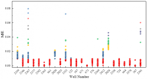
Figure 2. Relative errors of multiple single-well optimizations
As can be seen from Figure 2, the relative error of MSE of 1 is less than 0.08, that is, less than 8%. Statistics show that the errors between the predicted values and the measured ones obtained from many wells and measuring points are around 0.28 MPa. In 24 sample wells, the relative errors at all measuring points in 21 wells are less than 1%, that is, the errors at the measuring points in 87.5% of the wells are within 0.1 MPa. On the basis of this error range, the optimal parameters suitable for all wells in the block were selected, to ensure that the errors of the wells calculated from the selected parameters would be within a reasonable range.
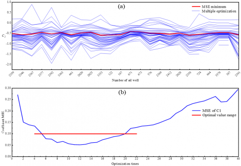
There are six parameters involved in the optimization of liquid holdup $H_l$. After the above-mentioned repeated single-well optimization, there are many sets of reasonable parameters for single wells, but applying a certain set of parameters for a certain well to the whole block will result in big errors. In order to obtain a set of reasonable parameters suitable for the current block, firstly, the six parameters obtained from multiple optimizations performed on all the sample wells were processed respectively. In the processing of C1, the values of C1 obtained from multiple optimizations on all the wells were sorted from large to small, and the set with the smallest MSE was selected from the sorted parameters, that is, the red curve shown in Figure 3(a), which is the best set for the 24 wells in the block, fluctuating within a certain numerical range. The remaining five parameters are processed in the same way.
In the screening process of the six parameters applicable to this block, it is impossible to obtain them all at the same time due to multiple optimizations. Therefore, these six parameters were selected according to the greedy principle. Moreover, in the selection process of the optimal parameters by the greedy lgorithm, due to factors such as different physical parameters of single wells, noise of measured data, and local convergence of the optimization algorithm, etc., if C1 is set at a single value, there may be no corresponding optimal correction coefficient in the selection process of C1-C6. To solve this problem, as shown in Figure 3(b), C1 values taken from both sides of a certain range were regarded as the optimal set of C1 values, and the set with the smallest MSE with respect to the above coefficient C1 as the center. The principle for determining the range is to ensure that at least one value can be obtained for the next correction coefficient. According to the greedy principle, other parameters were obtained in the same manner. The steps of how to screen all the coefficients are shown below.
(1) Sort the coefficients C1-C6 obtained through multiple optimizations on different wells in descending order respectively;
(2) Calculate the MSEs of all single optimization results for different coefficients of all the sample wells;
(3) Take a set of coefficient values with the smallest MSE as the center, select the values from both sides within a certain range of MSE, as the optimal result series for a certain correction coefficient.
(4) According to the greedy principle, starting from C1, select all the coefficients from C1 to C6 successively. Make sure that one or more corresponding coefficient combinations can be selected for each well.
Through the above screening, a set of optimal parameter series of C1-C6 suitable for the current block can be obtained, and each parameter contains 24 parameters suitable for all wells. The average value of 24 parameters is taken as the optimal value, that is to say, the optimal set of the six parameters is obtained. After screening and optimization, the optimal coefficient combination is as follows: C1 =-032, C2 =-0.060, C3 = 0.077, C4 = 2.36, C5 = 0.378, and C6 = 0.155.
Figure 3. (a) Statistical results of coefficient C1 after multiple optimizations on all the wells. (b) MSE of coefficient C1 after multiple optimizations
3.4 Verification and analysis
Considering that the production parameters of different wells vary greatly even in the same block, with the changes of production parameters, the non-optimized multiphase flow model may often suffer from very large prediction errors. In this case, whether the model can well adapt to the great changes in the production parameters of the block is the criterion for evaluating the robustness of the model. In order to test the applicability of the optimized model to the corresponding block and strata, five wells were randomly selected in the same block and strata at first, and wellbore pressure gradient tests were carried out on the selected wells to test the applicability and accuracy of the model. Meanwhile, the production parameters of the selected five wells were quite different. After several rounds of screening, the well depths of the selected five wells ranged between 3027m-3515m, the maximum wellhead pressure was 2.78 MPa, the minimum wellhead pressure 1.53 MPa, and the measured bottom hole pressure between 4.5 MPa -10 MPa. Accordingly, the gas-liquid ratio, which has great impact on the accuracy of the multiphase flow model in the wellbore, was between 200 and 5000 m3/m3. The optimization speed was also considered. Since the traditional method is manual and inefficient, it was not considered in this study. The effectiveness of the algorithm was verified mainly through comparison of the optimization speeds of SPSA and PSO [15].
Figure 4. (a) Comparison of running time between PSO and SPSA; (b)-(f) Model accuracy verification; (g) Maximum and minimum relative errors
In order to verify the efficiency of SPSA in the process of multiphase flow optimization, the SPSA and PSO algorithms were optimized 18 times each, and the average optimization time of multiple optimizations was taken as the optimization time of the algorithm, provided that the convergence conditions and other hardware conditions were the same. As shown in Figure 4 (a), the average convergence time of PSO was 34,000 ms, while that of SPSA 3400 ms, which was about 1/10 of the former. So when there is massive amount of measured data, the optimization efficiency can be increased.
In the process of gas lift design in area R of an oilfield in Kazakhstan, the relative errors in the prediction of the wellbore multiphase flow model should be no more than 15%, based on the field experience of multi-well gas lift design. When applied to gas lift design, the relative errors of the predicted values were within the desired range, and the design results could meet the actual needs and helped achieve a reasonable gas injection depth and high lifting efficiency. In order to ensure the properness of the verification results, four wells other than the sample ones were selected as the verification set, and the accuracy of the optimized model was verified by comparison of the prediction results obtained from the pre-optimized model and the optimized model and the measured ones.
As shown in Figures 4(b)-(f), regarding the prediction results of the Mukherjee-Brill model before optimization, only those obtained at the first three measuring points in Figure 4(d) and Figure 4(f) had an error of less than 15%. In Figure 4(d), the relative error at the fourth measuring point was not desired, and the predicted value was smaller than the measured one. The gas-lift valve designed based on this result will have a greater depth. The results obtained at the measuring points below 1000m in the well shown in Figure 4(b), (c) and (e) did not meet the precision requirements. Moreover, the predicted value at each measuring point was generally too large. Applying this result to the gas lift design will lead to an excessively small depth of a gas lift valve, which will result in an increase in the number of gas lift valves, and thus increase in cost and difficulty of operation. At the same time, it will also affect the lifting efficiency and make the output unable to meet the design requirement.
As shown in Figure 4(g), the results obtained from the optimized model all met the requirement that the relative error should be less than 15%. The maximum relative error of the four wells was 7.13%, with the predicted value being 0.158 MPa higher than the measured one, and the minimum relatively error was 0.01%, with the predicted value being 0.0003 MPa lower than the measured one. Gas lift design and gas lift condition diagnosis based on such predicted values can meet the prediction accuracy requirement for the multiphase flow model. Therefore, the SPSA algorithm can improve the efficiency, meet the accuracy requirement, and provide a fast and effective optimization solution for the field application.
(1) The optimization of the wellbore multiphase flow model based on the SPSA algorithm was studied in this paper. By optimizing the main influencing factors in the model, the efficient optimization of the model was realized. In practical application, it is able to meet the accuracy requirement of less than 15% for relative errors, which provides a feasible way for solving the optimization of the model based on massive measured data.
(2) The results show that the SPSA optimization algorithm has higher optimization efficiency than the traditional manual method and the PSO algorithm. Its optimization speed is about 10 times faster than that of the PSO algorithm, which can effectively ensure the timeliness of gas lift diagnosis and design.
(3) Through multiple optimizations and with the aid of the greedy algorithm in the selection of the optimal parameters for a block, the local convergence of SPSA algorithm can be effectively reduced, which makes the optimization result satisfactory.
The authors would like to acknowledge the support provided by the National Natural Science Foundation of China (Grant No.: 62173049) and the open fund of the Key Laboratory of Exploration Technologies for Oil and Gas Resources (Yangtze University), Ministry of Education (Grant No.: K2021-17).
|
SPSA |
Simultaneous Perturbation Stochastic Approximation |
|
PSO |
Particle Swarm Optimization |
|
SA |
Stochastic Approximation |
|
$\widehat{\boldsymbol{g}}_k$ |
Disturbance gradient |
|
$\boldsymbol{u}_k$ |
Optimal control vector corresponding to the k-th step |
|
$\varepsilon_k$ |
Disturbance step |
|
$\boldsymbol{\delta}_k$ |
N-dimensional random disturbance vector |
|
$a_k$ |
Gain value |
|
$c_k$ |
Disturbance steps |
|
$d p / d z$ |
Total pressure drop, MPa/m |
|
$(d p / d z)_g$ |
Heavy pressure drop, MPa⁄m |
|
$(d p / d z)_f$ |
Frictional pressure drop, MPa/m |
|
$(d p / d z)_a$ |
Acceleration pressure drop, MPa/m |
|
$f_m$ |
Friction coefficient of the gas-liquid two-phase mixture |
|
C1~C6 |
Coefficient combination |
|
v |
Average velocity of mixture, m/s |
|
D |
Pipe diameter |
|
$\mathrm{H}_l$ |
Liquid holdup, m3/m3 |
|
$N_{v l}$ |
Liquid phase velocity criterion |
|
$N_{v g}$ |
Gas phase velocity criterion |
|
$N_l$ |
Liquid viscosity criterion |
|
MSE |
Mean Square Error |
|
$\bar{y}_i$ |
Measured value |
|
$y_i$ |
Predicted value |
|
n |
Number of measuring points |
|
Greek symbols |
|
|
$\rho_m$ |
Density of the mixture,Kg/m3 |
|
$\rho_m$ |
Liquid-phase density, Kg/m3 |
|
$\rho_g$ |
Gas phase density, Kg/m3 |
|
Subscripts |
|
|
$k$ |
Number of iterations |
|
$m$ |
Mixture |
|
$l$ |
Liquid phase |
|
$g$ |
Gas phase |
|
$v l$ |
Liquid phase velocity |
|
$v g$ |
Gas phase velocity |
|
$a$ |
Acceleration |
|
$f$ |
Friction |
|
$g$ |
Gravitational acceleration |
[1] Mukherjee, H., Brill, J.P. (1985). Pressure drop correlations for inclined two-phase flow. Journal of Energy Resources Technology, 107(4): 549-554. https://doi.org/10.1115/1.3231233
[2] Mukherjee, H., Brill, J.P. (1983). Liquid holdup correlations for inclined two-phase flow. Journal of Petroleum Technology, 35(5): 1003-1008. https://doi.org/10.2118/10923-PA
[3] Beggs, D.H., Brill, J.P. (1973). A study of two-phase flow in inclined pipes. Journal of Petroleum technology, 25(5): 607-617. https://doi.org/10.2118/4007-PA
[4] Aziz, K., Govier, G.W. (1972). Pressure drop in wells producing oil and gas. Journal of Canadian Petroleum Technology. https://doi.org/10.2118/72-03-04
[5] Orkiszewski, J. (1967). Predicting two-phase pressure drops in vertical pipe. Journal of Petroleum Technology, 19(6): 829-838. https://doi.org/10.2118/1546-PA
[6] Hagedorn, A.R., Brown, K.E. (1965). Experimental study of pressure gradients occurring during continuous two-phase flow in small-diameter vertical conduits. Journal of Petroleum Technology, 17(4): 475-484. https://doi.org/10.2118/940-PA
[7] Dong, Y., Liao, R.Q., Luo, W., Li, M.X. (2022). An improved pressure drop prediction model based on Okiszewski’s model for low gas-liquid ratio two-phase upward flow in vertical pipe. International Journal of Heat and Technology, 40(1): 17-22. https://doi.org/10.18280/ijht.400103
[8] Wen Y., Wu Z.H., Wang J.L., Wu J., Yin Q.G., Luo W. (2017). Experimental study of liquid holdup of liquid-gas two-phase flow in horizontal and inclined pipes, International Journal of Heat and Technology, 35(4): 713-720. https://doi.org/ 10.18280/ijht.350404
[9] Ansari, A.M., Sylvester, N.D., Sarica, C., Shoham, O., Brill, J.P. (1994). A comprehensive mechanistic model for upward two-phase flow in wellbores. SPE Production & Facilities, 9(2): 143-151. https://doi.org/10.2118/20630-MS
[10] Spall, J.C. (1998). Implementation of the simultaneous perturbation algorithm for stochastic optimization. IEEE Transactions on aerospace and electronic systems, 34(3): 817-823. https://doi.org/10.1109/7.705889
[11] Spall, J.C. (1998). An overview of the simultaneous perturbation method for efficient optimization. Johns Hopkins Apl Technical Digest, 19(4): 482-492.
[12] Zhao, H., Cao, L., Li, Y., Yao, J. (2011). Production optimization of oil reservoir based on an improved simultaneous perturbation stochastic approximation algorithm. Acta Petrolei Sinica, 32(6): 1031-1036. https://doi.org/10.7623/syxb201106016
[13] Zhang, K., Zhang, X., Zhang, L. (2017). A novel approach for optimization of polymer-surfactant flooding based on simultaneous perturbation stochastic approximation algorithm. Journal of China University of Petroleum (Edition of Natural Science), 41(5): 102-109. https://doi.org/10.3969/j.issn.1673-5005.2017.05.012
[14] Kong, X.S., Guo, J.M., Zheng, D.B., Yang, J.F., Zhang, J., Fu, W. (2020). An Improved-SPSA quality control method for medium voltage insulator SPSA. Journal of Chemical Engineering of Chinese Universities, 34: 1500-1510. https://doi.org/10.3969/j.issn.1003-9015.2020.06.022
[15] Kennedy, J., Eberhart, R. (1995). Particle swarm optimization. In Proceedings of ICNN'95-international conference on neural networks, 4: 1942-1948. https://doi.org/10.1007/978-0-387-30164-8_630
[16] Yang, W., Li, Q.Q. (2004). Overview of particle swarm optimization algorithms. Strategic Study of CAE, (25): 87-94. https://doi.org/10.3969/j.issn.1009-1742.2004.05.018