Ling Jin | Xiaoli Liu* | Yan Jiang | Yali Guan | Zhaoying Liu
© 2022 IIETA. This article is published by IIETA and is licensed under the CC BY 4.0 license (http://creativecommons.org/licenses/by/4.0/).
OPEN ACCESS
The accurate prediction of the short-term heat load trend of buildings helps to prevent energy waste. Combinatory prediction methods need to be studied, as the processing of real-time data series of heat supply and the accurate prediction of short-term trend are more and more demanded by different heating districts and independent buildings. Therefore, this study explores the application of optimal combinatory mathematics model in heat load trend prediction. Firstly, feature extraction was performed on the historical weather data at the locality of the building and the historical data on heat load, creating a short-term trend prediction dataset with days as the unit, and an ultra-short-term trend prediction dataset with hours as the unit. On this basis, a combinatory mathematics model was created for heat load trend prediction. Furthermore, the authors detailed the principles of the two methods, namely, extreme gradient boosting tree (EGBT) and support vector regression (SVR), and explains the combination pattern of the single models in the combinatory model. Then, the weights were optimized by the simulated annealing (SA) algorithm, and the steps of the combinatory model were presented. The proposed model was proved effective through experiments.
combinatory mathematics model, heat load, trend prediction
Heat load accounts for a large proportion of building energy consumption, making it imperative to save heating energy [1-8]. The accurate prediction of the short-term heat load trend of buildings helps to avoid energy waste, and provides a promising way to precisely regulate building energy based on energy demand [9-13]. With the expansion of heating scale and the growing complexity of heating data, there is a growing demand for processing the real-time data series of heat supply and predicting the short-term trend accurately for different heating districts and independent buildings [14-20]. The single prediction model with specific mathematical assumptions and applicable conditions can hardly meet the strict mathematical preconditions and hypotheses concerning the load trend prediction of actual heat supply projects in the background of big data [21-24]. To realize refined planning and decision-making of energy heat supply, the combinatory prediction method came into being, providing an effective way to elevate the accuracy of trend prediction.
The accurate description and prediction of the heat load of buildings connected to the district heating (DH) network is crucial to the effective operation of these systems. Lumbreras et al. [25] proposed a new data-driven model to describe and predict the heating demand of buildings connected to the DH network. After analyzing the heat load curve, these authors put forward a model that combines supervised clustering and multiple regression. The model utilizes four climate variables, including outdoor ambient temperature, global solar radiation, wind speed, and wind direction, and gives consideration to the time factor and the data from smart meters. The model was designed for deployment in large building complexes and to predict heat load without considering the construction features or end use of the building. Gong et al. [26] developed an Informer-based DHS framework for heat load prediction. To measure the performance of Informer in heat load prediction, four prediction models, namely, the autoregressive integrated moving average model (AIMA), the multilayer perceptron (MLP), the recurrent neural network (RNN), and the long-short-term memory network (LSTM), were established for comparison. Taking the historical heat load, outdoor temperature, relative humidity, wind speed and air quality index of a DHS in Tianjin as input features, the performance of the five prediction strategies was evaluated comprehensively. Zhang et al. [27] applied TimeGAN to the heating field for the first time to increase the data volume and improve the prediction accuracy of the model. The results show that, after using TimeGAN in the early stage of heating, the prediction error was reduced by 50%, while the coefficient of the variation of the root mean square error (CV-RMSE) could reach 0.0405. The prediction accuracy peaked when the synthetic data was three times the original data. Castellini et al. [28] proposed a method to generate simple and interpretable heat load prediction models, and applied this method to real datasets, providing new insights into this application area. Their method incorporates multi-equation multiple linear regression (MLR) and forward variable selection, and generates a sparse equation for each hour of each day of the week. Wang et al. [29] presented a layer transfer model and a combinatory transfer model for heat load prediction in district heating stations. Experimental protocols were developed to simulate cross-annual and cross-site scenarios, and the actual data were collected to serve the experiments. In the cross-site scenario, their model achieved good prediction performance, when the training data was insufficient.
Scholars at home and abroad have tried to develop trend prediction algorithms suitable for the heat load of buildings. The common algorithms fall into software simulation, statistical analysis, machine learning, and deep learning. The above methods face multiple common problems: the time sequence between data is considered insufficiently, the convergence is slow and unstable, the results are affected by too many parameters, and the model optimization takes a long time. Therefore, this study explores the application of optimal combinatory mathematics model in heat load trend prediction. Section 2 extracts the features from the historical weather data at the locality of the building and the historical data on heat load, creating a short-term trend prediction dataset with days as the unit, and an ultra-short-term trend prediction dataset with hours as the unit. On this basis, a combinatory mathematics model was created for heat load trend prediction. Furthermore, the authors detailed the principles of the two methods, namely, extreme gradient boosting tree (EGBT) and support vector regression (SVR), and explains the combination pattern of the single models in the combinatory model. Section 3 optimizes the weights by the simulated annealing (SA) algorithm, and illustrates the steps of the combinatory model. The proposed model was proved effective through experiments.
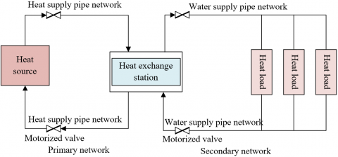
Figure 1. Structure of heat supply control system
Figure 2. Heat load regulation principle of the secondary network
Figure 1 shows the structure of the heat supply control system. In the primary network of the system, the heating pipe network sends the hot water heated by the heating source to the heat exchange stations for heat energy exchange, and then returns the hot water after the heat energy exchange and cooling is completed to the heating source for reheating. In the secondary network, the heating pipe network sends the cold water from the heat load (building) to the heat exchange stations for heat exchange, and then sends the cold water after the heat exchange and temperature rise to the heat load. Figure 2 shows the heat load regulation principle of the secondary network. According to the heat balance equation, the regulator needs to control the flow regulating valve based on the heating temperature threshold. The heating temperature threshold here is directly related to the heat load demand. The accurate prediction of the heat load trend is the premise for realizing the real-time and accurate control of the actual water supply temperature.
Feature extraction is the decisive factor for the accuracy of heat load trend prediction model. The feature extraction for heat load prediction aims to extract valuable parameters for prediction from the historical heating data before making predictions, and import them to train the prediction model. This paper mainly extracts and processes features of the historical data on the weather and heat load of the locality of the building.
The weather file contains many parameters, including the air temperature at 1.5 m above the ground, dew point temperature, ratio of water vapor pressure to saturated water vapor pressure, direct solar radiation, diffuse solar radiation, wind speed and direction at 11 m above the ground, atmospheric pressure, and the degree to which clouds obscure the view of the sky. The above parameters mainly affect the heat exchange between the building envelope and the indoor environment, and indirectly affect the heat load of the building. The internal disturbances affecting the heat load mainly include the operation of electrical equipment and indoor activities. Considering the thermal inertia transmitted by the above parameter changes, it is necessary to fully consider the heat load response with a certain delay. A raw dataset is constructed based on all of the above collectible variables.
There are two target scales for building heat load trend prediction: the short-term (1-3 days in the future) or the ultra-short-term (15 min-4 h in the future). This section further processes the original dataset, and divides it into a short-term trend prediction dataset with day as the unit and an ultra-short-term trend prediction dataset with hour as the unit.
Our combinatory mathematics model for heat load trend prediction synthetizes EGBT and SVR. The principles and combinatory pattern of the two methods are detailed below.
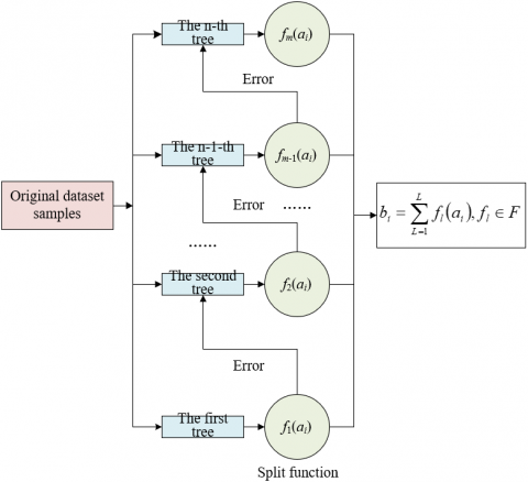
Figure 3 shows the principle of EGBT. It is assumed that m trees are trained in EGBT. Then, the EGBT can be expressed as follows:
$b_i=\sum_{l=1}^m f_l\left(a_i\right), f_l \in F$ (1)
The base classifier of EGBT is a regression tree model, which is represented by a sub-function f of the function space F. Then, the entire set of regression trees can be represented by F. The objective function of EGBT can be defined as:
$P Q(\omega)=\sum_{i=1}^m k\left(b_i, b_i\right)+\sum_{i=1}^l \Xi\left(f_i\right)$ (2)
Figure 3. Principle of EGBT
EGBT needs to obtain all decision trees through iterative operations, i.e., the l-1-th iteration results are further iteratively trained to generate the l-th decision tree. Let bi(l) be the prediction result generated in the l-th time. Then, the iterative process can be expressed as:
$b_i^{(0)}=0$
$b_i^{(1)}=f_1\left(a_i\right)=b_i^{(0)}+f_1\left(a_i\right)$
$b_i^{(2)}=f_1\left(a_i\right)+f_2\left(a_i\right)=b_i^{(1)}+f_2\left(a_i\right)$
$\cdots$
$b_i^{(l)}=\sum_{r=1}^l f_r\left(a_i\right)=b_i^{(l-1)}+f_l\left(a_i\right)$ (3)
The objective function of the prediction error of the l-th iteration can be expressed as:
$P Q^l=\sum_{i=1}^m k\left(b_i, b_i^{(l)}\right)+\sum_{i=1}^l \Xi\left(f_i\right)=\sum_{i=1}^m k\left(b_i, b_i^{(l-1)}+f_l\left(a_i\right)\right)+\Xi\left(f_l\right)+C O$ (4)
The secondary Taylor expansion of the loss function can be expressed as:
$P Q^{(l)}=\sum_{i=1}^m\left[k\left(b_i, b_i^{(l-1)}\right)+h_i f_l\left(a_i\right)+\frac{1}{2} g_i f_l^2\left(a_i\right)\right]+\Xi\left(f_l\right)+C O$ (5)
where, hi and gi can be respectively defined by:
$h_i=\partial_{b_i^{(i-1)}} k\left(b_i, b_i^{(l-1)}\right)$ (6)
$g_i=\partial_{b_i^{(i-1)}}^2 k\left(b_i, b_i^{(l-1)}\right)$ (7)
By deleting the less influential constant, the objective function of the expanded L-th iteration can be given as:
$P Q^{(l)}=\sum_{i=1}^m\left[h_i f_l\left(a_i\right)+\frac{1}{2} g_i f_l^2\left(a_i\right)\right]+\Xi\left(f_l\right)$ (8)
Formulas (7) and (8) show that hi and gi determine the value of the objective function of prediction error. Therefore, EGBT can set various loss functions according to the demand predicted by the actual heat supply project. Taking the squared loss function as an example, the following objective function can be obtained:
$P Q^{(l)}=\sum_{i=1}^m\left(b_i-\left(b_i^{(l-1)}+f_l\left(a_i\right)\right)\right)^2+\sum_{i=1}^l \Xi\left(f_i\right) r$
$\sum_{i=1}^m\left[2\left(b_i^{(l-1)}-b_i\right) f_l\left(a_i\right)+f_l\left(a_i\right)^2\right]+\Xi\left(f_l\right)+C O$ (9)
The SVR in the combinatory mathematics model can be expressed as:
$b(A)=Q^T \zeta(A)+\varsigma$ (10)
where, A is the features of the original data input of the model; ς is the constant term; Q is the weight vector; b(A) is the prediction value; ζ(.) is the kernel method for mapping the original data A to the linear space ζ(A).
The cost function of SVR needs to ensure that the decision boundary c=2/|q| is maximum, i.e., the cumulative prediction error and structural error are minimized simultaneously. Then, the cost function can be expressed as:
$\frac{1}{2} \sum_{m=1}^M\left|b_m-b_m^{\prime}\right|^2+\frac{\mu}{2}\|q\|^2$ (11)
where, bm is the value predicted by the learning algorithm; b'm is the actual value of the data point; μ is the regularization parameter.
To ensure that SVR has a sparse solution for building heat load trend prediction, this paper introduces a non-negative insensitive parameter ῶ to correct the quadratic error function |bm-b'm|2. If the difference between the prediction result bm and the prediction target b'm is smaller than ῶ, then the error is zero. The corrected error function can be given by:
$W C_{\mathrm{E}}\left(b(A)-b^{\prime}\right)=\left\{\begin{array}{l}0, \text { if }\left|b(A)-b^{\prime}\right|<\tilde{\omega} \\ \left|b(A)-b^{\prime}\right|-\tilde{\omega}, \text { otherwise }\end{array}\right.$ (12)
Let D be the reciprocal of the regularization parameter. By combining formulas (40) and (41), the decision boundary error function that requires minimum regularization can be obtained:
$D \sum_{m=1}^M W C_{\varepsilon}\left(b_m-b_m^{\prime}\right)+\frac{1}{2}\|q\|^2$ (13)
This paper introduces slack variables to optimize the SVR, so that the model allows a few prediction results outside the decision boundary. Each parameter sample Am needs two slack variables Φm and Φ'm. If Φm>0 and Φ'm=0, then Am corresponds to a point outside the model regression decision boundary; If Φm=0 and Φ'm=0, then Am corresponds to a point inside that boundary.
For a sample without slack variables to fall within the decision boundary, b(Am)-ῶ≤b'm≤b(Am)+ῶ is the necessary condition:
$b_m^{\prime} \leq b\left(A_m\right)+\epsilon+\Phi_m$ (14)
$b_m^{\prime} \geq b\left(A_m\right)-\epsilon-\Phi_m^{\prime}$ (15)
Introducing positive slack variables Φm and Φ'm, the cost function of the SVR can be expressed as:
$D \sum_{m=1}^M\left(\Phi_m+\Phi_m^{\prime}\right)+\frac{1}{2}\|q\|^2$ (16)
Let A be the input eigenvector extracted from the original dataset, which is constructed from the collectable variable data; b be the short-term or ultra-short-term heat load predicted for the building. Then, the heat load prediction model based on the improved SVR can be expressed as:
$b(A)=Q^T \zeta(A)+\zeta$ (17)
The above analysis shows that the selection of kernel function and penalty function D significantly affects the prediction performance of the model. Let ε be the width parameter of the function. This paper chooses the Gaussian function as the kernel function of the improved SVR:
$\zeta\left(a_i\right)_i=\exp \left(-\frac{\left\|a_i-k^{(i)}\right\|^2}{2 \varepsilon^2}\right)$ (18)
The above formula shows that the kernel function is a monotonic function of the Euclidean distance from any sample ai to the center k(i) of a sample. The closer ai is to k(i), the closer the value of ζ(ai)i is to 1. The further ai is from k(i), the closer the value of ζ(ai)i is to 0. ε is used to control the range of radial effect of the kernel function. The larger the ε, the smaller the impact of the changing distance between ai and k(i) on the value of ζ(ai)i. Then, the smoothness of the function will be improved.
This paper combines EGBT and SVR to extract the nonlinear features of the short-term trend prediction dataset and the ultra-short-term trend prediction dataset in a comprehensive manner. In this way, the strength of the two models was given full play, and the combinatory prediction model was optimized to predict the heat load trend. The combination protocol is to weigh and summarize the prediction results of the two models:
$b=\beta g_1+(1+\beta) g_2$ (19)
where, g1 and β are the prediction result and weight coefficient of EGBT, respectively; g2 and 1-β are the prediction result and weight coefficient of SVR, respectively; b is the heat load trend predicted by the optimal combinatory model.
Since β and 1-β are difficult to assign, this paper optimizes the weights based on the SA algorithm, a global optimizer. A sufficiently slow annealing can promote the effective convergence of the heat load trend prediction to the global optimal solution. The flow of the SA is as follows:
Step 1. Initialize the annealing temperature χl, and the initial solution a0.
Figure 4. Prediction flow of heat load for the optimal combinatory model
Table 1. Performance of prediction models with different penalty coefficients and kernel function widths
|
Kernel function width Penalty coefficient |
2-11 |
2-10 |
2-9 |
2-8 |
2-7 |
2-6 |
2-5 |
2-4 |
2-3 |
2-2 |
|
25 |
0.62 |
0.63 |
0.76 |
0.69 |
0.62 |
0.68 |
0.52 |
0.42 |
0.31 |
0.12 |
|
26 |
0.66 |
0.74 |
79 |
0.75 |
0.79 |
0.65 |
0.67 |
0.58 |
0.45 |
0.36 |
|
27 |
0.72 |
0.79 |
0.72 |
0.71 |
0.72 |
0.74 |
0.63 |
0.62 |
0.59 |
0.42 |
|
28 |
0.74 |
0.72 |
0.77 |
0.73 |
0.74 |
0.70 |
0.75 |
0.69 |
0.51 |
0.55 |
|
29 |
0.79 |
0.71 |
0.71 |
0.77 |
0.73 |
0.73 |
0.79 |
0.74 |
0.67 |
0.58 |
|
210 |
0.75 |
0.70 |
0.74 |
0.74 |
0.71 |
0.78 |
0.71 |
0.72 |
0.78 |
0.62 |
|
211 |
0.72 |
0.76 |
0.76 |
0.70 |
0.75 |
0.75 |
0.78 |
0.70 |
0.71 |
0.67 |
|
212 |
0.74 |
0.72 |
0.78 |
0.72 |
0.78 |
0.71 |
0.75 |
0.78 |
0.74 |
0.79 |
|
213 |
0.78 |
0.74 |
0.73 |
0.75 |
0.71 |
0.79 |
0.73 |
0.73 |
0.77 |
0.75 |
|
214 |
0.76 |
0.78 |
0.71 |
0.78 |
0.75 |
0.77 |
0.71 |
0.79 |
0.75 |
0.71 |
Step 2. Randomly select a new feasible solution a' in the neighborhood of solution a, and calculate the difference Δg= g(a')-g(a) between objective function values g(a') and g(a). When the probability satisfies min{1,S=exp(-Δg/Rl)}>random[0,1], accept a'.
Step 3. Repeat Step 2 at the temperature χl until reaching the equilibrium state.
Step 4. Perform the annealing operation Rl+1=DRl,l←l+1, D$\in$(0,1). If the maximum iterative value is reached, or the error meets the condition, end the annealing operation; otherwise, return to Step 2.
Figure 4 displays the prediction flow of the heat load by the optimal combinatory model. This model is executed in the following steps:
Step 1. Preprocess and normalize the original dataset, and build a training set and a test set based on the short-term trend prediction dataset and the ultra-short-term trend prediction dataset by different ratios.
Step 2. Establish EGBT and optimize SVR to obtain their predicted heat load trends g1 and g2.
Step 3. Initialize the annealing temperature χl, set the initial solution a0, and define the lower bound of temperature, maximum number of iterations, and other parameters of the SA.
Step 4. Set the objective function for the prediction error of the optimal combinatory model, i.e., the ratio of the prediction error and the actual heat load.
Step 5. Calculate the initial value of the prediction error objective function based on a0.
Step 6. Generate random disturbances in model execution, and compute the value of the prediction error objective function based on the new solution. If the error is smaller than zero, accept the new solution; if the error is greater than zero, calculate the probability according to the preset rule and threshold, and judge whether the poorer solution is acceptable.
Step 7. If the prediction error stabilizes or the number of iterations reaches the maximum, terminate the iterations, and output the optimal β and 1-β; otherwise, return to Step 5.
Step 8. Compute the heat load trend predicted by the optimal combinatory model according to the optimal β and 1-β.
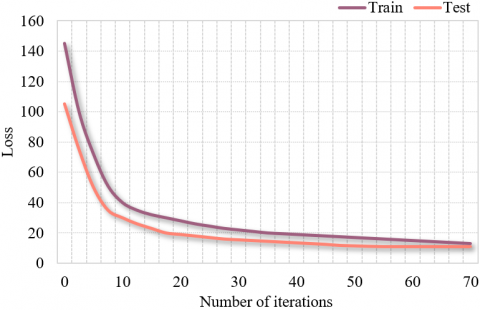
As mentioned before, the original dataset was developed based on the historical weather data at the locality of the building and the historical data on heat load. The dataset was imported to the proposed heat load trend prediction model. The obtained training curve is displayed in Figure 5. It can be seen that, the training and test errors of EGBT gradually decreased with the growing number of iterations, and the loss tended to be stable after 50 iterations.
To obtain the most ideal SVR prediction model, this paper determines the penalty coefficient and kernel function width through grid search. The value range of the penalty coefficient and kernel function width was determined as {31, 32, …, 237} and {2−10, 2−9, …, 2−2}, respectively. The original dataset was divided into ten parts, and used to train the ten prediction models. The idealness of the SVR prediction model was characterized by the mean prediction accuracy of all prediction models. Table 1 reports the performance of the prediction models with different penalty coefficients and kernel function widths. Eventually, the penalty coefficient and kernel function width of the SVR for real heat load prediction were determined as 223 and 2−6, respectively. The data on the weather and heat load of the locality of the building were collected for the future 24 h and the past 6 h. Then, the data of the first 1 h and the past 6 h were extracted to import to the SVR to obtain the predicted heat load trend of the first 1 h. Next, the data of the second hour and the past 6 h were extracted to predict the heat load trend. The above steps were repeated to obtain the complete heat load prediction data of the coming 24 h.
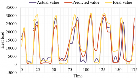
To verify the effectiveness of the combinatory model for heat load trend prediction, a single prediction model was selected as a comparison model. Table 2 compares the prediction results. It can be seen that the mean absolute percentage error (MAPE) of the combinatory model for the heat load was 0.88%, which was 3.2% and 1.67% lower than that of EGBT and SVR alone, respectively. The mean absolute error (MAE) of the combinatory model for the heat load was 181.36 kW, and 171.24 kW lower than that of EGBT and SVR alone, respectively. The root mean square error (RMSE) of the combinatory model for the heat load was 191.47 kW, and 152.97 kW lower than that of EGBT and SVR alone, respectively. It can be seen that the combinatory model predicted the trend of heat load well, which is largely in line with the actual situation of the project. In addition, the prediction effect of the combinatory model was much better than EGBT and SVR alone. This testifies the effectiveness and superiority of the combinatory model in heat load trend prediction. Statistical analysis was performed to extract the data for predicting heat load trend from the historical weather and heat load data of the locality of the target building from December 2nd to December 8th. Figure 6 shows the actual heat load, predicted heat load, and ideal heat load of the building in that period. Comparing the actual and predicted heat loads of the building, it can be seen that the heat load trend prediction of the model was rather good in most of the period. Thus, the model can effectively and reasonably predict the heat load, using the said historical data.
Figure 5. EGBT training curve
Table 2. Comparison of heat load prediction errors of different models
|
Date |
Model |
MAPE/% |
MAE/kW |
RMSE/kW |
|
December 2nd |
EGBT |
2.68 |
258.14 |
294.58 |
|
SVR |
2.14 |
269.27 |
274.15 |
|
|
Combinatory model |
1.62 |
115.35 |
163.27 |
|
|
December 3rd |
EGBT |
2.58 |
169.82 |
248.61 |
|
SVR |
3.95 |
372.16 |
348.27 |
|
|
Combinatory model |
1.62 |
142.57 |
196.05 |
|
|
December 4th |
EGBT |
2.84 |
269.63 |
357.28 |
|
SVR |
3.67 |
358.37 |
311.62 |
|
|
Combinatory model |
1.95 |
162.42 |
147.28 |
|
|
December 5th |
EGBT |
2.38 |
174.28 |
162.95 |
|
SVR |
2.11 |
268.15 |
238.51 |
|
|
Combinatory model |
0.85 |
52.47 |
85.62 |
Figure 6. Predicted heat loads from December 2nd to December 8th
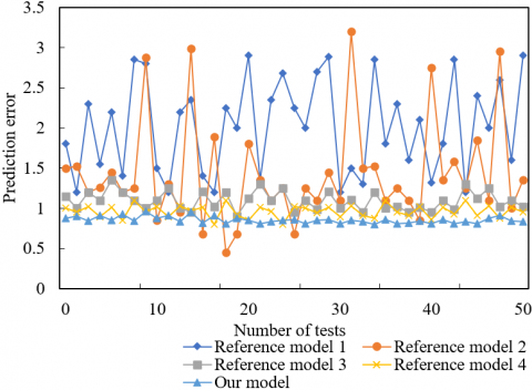
Figure 7. Oscillations of prediction results of different models
The above figure shows that the heat load of the building at night was higher during the study period, mainly because the model ignores less sunlight, low temperature, and less indoor activities at night. The neglection of these factors suppresses the prediction accuracy. In addition, the above experiments show that the proposed combinatory model does not need the details of the actual building to predict the heat load. It only needs the historical data on the local weather and the building’s heat load in the past 6h. This means the model has a strong generalization ability, and is feasible for predicting the heat load of the actual project.
To further verify the effectiveness of the combinatory model, this paper selects four reference models for comparative experiments on prediction stability. The reference models include CNN+LSTM (reference model 1), LSSVM+ARIMA (reference model 2), and LSSVM+K nearest neighbors (Reference model 3), and our model without SA (reference model 4). Figure 7 compares the oscillation of the prediction results of different models.
As shown in Figure 7, the prediction result of our model oscillates 5% less intensively than that of any reference model. The prediction stability was enhanced significantly, which fully demonstrates the superiority of EGBT and SVR combinatory model in heat load prediction. The proposed model was compared with the model without SA in terms of the prediction oscillation, aiming to prove that the combinatory weighting of SA stabilizes the prediction. The comparison shows that the SA can enhance the stability of the prediction by the combinatory model, and can be widely applied to optimize the combinatory prediction model for the heat load in actual projects.
This research explores the application of optimal combinatory mathematics model in heat load trend prediction. Firstly, feature extraction was performed on the historical weather data at the locality of the building and the historical data on heat load, creating a short-term trend prediction dataset with days as the unit, and an ultra-short-term trend prediction dataset with hours as the unit. On this basis, a combinatory mathematics model was created for heat load trend prediction. Furthermore, the authors detailed the principles of the two methods, EGBT and SVR, and explains the combination pattern of the single models in the combinatory model. Then, the weights were optimized by the SA, and the steps of the combinatory model were presented. Through experiments, the EGBT training curve was drawn, and the SVR prediction effects with different penalty coefficients and kernel function widths. The heat load of the target building in the coming 24 h was obtained completely. Finally, four reference models were selected to comparatively test the prediction stability. The results show that the combinatory model is effective, and the combinatory weighting of the SA is effective.
[1] Zhao, A., Mi, L., Xue, X., Xi, J., Jiao, Y. (2022). Heating load prediction of residential district using hybrid model based on CNN. Energy and Buildings, 266: 112122. https://doi.org/10.1016/j.enbuild.2022.112122
[2] Huang, X., Xu, Z., Sun, et al. (2018). Heat and power load dispatching considering energy storage of district heating system and electric boilers. Journal of Modern Power Systems and Clean Energy, 6(5): 992-1003. https://doi.org/10.1007/s40565-017-0352-6
[3] Zgraja, J. (2018). Susceptibility of the LLC resonance generator for induction heating on changes in load parameters caused by heating the charge. In 2018 Conference on Electrotechnology: Processes, Models, Control and Computer Science (EPMCCS), Kielce, Poland, pp. 1-5. https://doi.org/10.1109/EPMCCS.2018.8596509
[4] Du, W., Zeng, M., Li, Y., Zhong, S., Wang, X. (2020). The heating load control method of load aggregators based on cluster analysis. In 2020 12th IEEE PES Asia-Pacific Power and Energy Engineering Conference (APPEEC), Nanjing, China, pp. 1-6. https://doi.org/10.1109/APPEEC48164.2020.9220357
[5] Yang, Y., Wang, F., Yan, G., Mu, G., Zhang, L. (2020). The regulating characteristic analysis for distributed electric heating load in Northern China. In 2020 IEEE Sustainable Power and Energy Conference (iSPEC), Chengdu, China, pp. 187-192. https://doi.org/10.1109/iSPEC50848.2020.9350994
[6] Waite, M., Modi, V. (2020). Electricity load implications of space heating decarbonization pathways. Joule, 4(2): 376-394. https://doi.org/10.1016/j.joule.2019.11.011
[7] Han, J., Ma, G., Hu, S., et al. (2018). Analysis of electric heating load characteristics in south Hebei power grid. In 2018 2nd IEEE Conference on Energy Internet and Energy System Integration (EI2), Beijing, China, pp. 1-5. https://doi.org/10.1109/EI2.2018.8582155
[8] Streicher, K.N., Schneider, S., Patel, M.K. (2020). Estimation of load curves for large-scale district heating networks. In IOP Conference Series: Earth and Environmental Science, 588(5): 052032. https://doi.org/10.1088/1755-1315/588/5/052032
[9] Kral, E., Kostalova, A., Capek, P., Vasek, L. (2018). Algorithm for central heating heat load modelling. In 2018 International Conference on Computational Science and Computational Intelligence (CSCI), Vegas, NV, USA, pp. 1438-1439. https://doi.org/10.1109/CSCI46756.2018.00279
[10] Li, B., Yang, D., Sun, Y., Liu, G., Fu, J., Liu, C. (2022). Blockchain-based smart contract enabling electric heating load participate in demand response. In 2022 7th Asia Conference on Power and Electrical Engineering (ACPEE), Hangzhou, China, pp. 507-512. https://doi.org/10.1109/ACPEE53904.2022.9783844
[11] Jeong, S.H., Jin, J.I., Park, H.P., Jung, J.H. (2022). Enhanced load adaptive modulation of induction heating series resonant inverters to heat various-material vessels. Journal of Power Electronics, 22: 1020-1032. https://doi.org/10.1007/s43236-022-00409-x
[12] Li, G., Zhou, C., Li, R., Liu, J. (2022). Heat load forecasting for district water-heating system using locality-enhanced transformer encoder. In Proceedings of the Thirteenth ACM International Conference on Future Energy Systems, pp. 440-441. https://doi.org/10.1145/3538637.3538751
[13] Wang, H.J., Jin, T., Wang, H., Su, D. (2022). Application of IEHO–BP neural network in forecasting building cooling and heating load. Energy Reports, 8: 455-465. https://doi.org/10.1016/j.egyr.2022.01.216
[14] Liu, J., Wang, X., Zhao, Y., Dong, B., Lu, K., Wang, R. (2020). Heating load forecasting for combined heat and power plants via strand-based LSTM. IEEE Access, 8: 33360-33369. https://doi.org/10.1109/ACCESS.2020.2972303
[15] Finkenrath, M., Faber, T., Behrens, F., Leiprecht, S. (2022). Holistic modelling and optimisation of thermal load forecasting, heat generation and plant dispatch for a district heating network. Energy, 250: 123666. https://doi.org/10.1016/j.energy.2022.123666
[16] Bianchi, F., Masillo, F., Castellini, A., Farinelli, A. (2020). XM_HeatForecast: Heating load forecasting in smart district heating networks. In International Conference on Machine Learning, Optimization, and Data Science, Siena, Italy, pp. 601-612. https://doi.org/10.1007/978-3-030-64583-0_53
[17] Idowu, S., Saguna, S., Åhlund, C., Schelén, O. (2016). Applied machine learning: Forecasting heat load in district heating system. Energy and Buildings, 133: 478-488. https://doi.org/10.1016/j.enbuild.2016.09.068
[18] Guan, N., Luan, T., Jiang, G., Liu, Z.G., Zhang, C.W. (2016). Influence of heating load on heat transfer characteristics in micro-pin-fin arrays. Heat and Mass Transfer, 52(2): 393-405. https://doi.org/10.1007/s00231-015-1565-8
[19] Sajjadi, S., Shamshirband, S., Alizamir, M., et al. (2016). Extreme learning machine for prediction of heat load in district heating systems. Energy and Buildings, 122: 222-227. https://doi.org/10.1016/j.enbuild.2016.04.021
[20] Qu, F., Sun, D., Bai, J., Zuo, G., Yan, C. (2018). Numerical investigation of blunt body’s heating load reduction with combination of spike and opposing jet. International Journal of Heat and Mass Transfer, 127: 7-15. https://doi.org/10.1016/j.ijheatmasstransfer.2018.06.154
[21] Sarnago, H., Lucía, Ó., Burdío, J.M. (2018). FPGA-based resonant load identification technique for flexible induction heating appliances. IEEE Transactions on Industrial Electronics, 65(12): 9421-9428. https://doi.org/10.1109/TIE.2018.2823687
[22] Swhli, K.M.H., Jovic, S., Arsic, N., Spalevic, P. (2017). Detection and evaluation of heating load of building by machine learning. Sensor Review, 38(1): 99-101. https://doi.org/10.1108/SR-07-2017-0139
[23] Ploskić, A., Wang, Q. (2018). Evaluating the potential of reducing peak heating load of a multi-family house using novel heat recovery system. Applied Thermal Engineering, 130: 1182-1190. https://doi.org/10.1016/j.applthermaleng.2017.11.072
[24] Li. G., Song, B.Y., Zhang, Z., Wang, H., Wang, J.H. (2016). Influences of side load and heating orientation on critical heat flux in a rectangular groove. Journal of Aerospace Power, 31(1): 203-210.
[25] Lumbreras, M., Garay-Martinez, R., Arregi, B., Martin-Escudero, K., Diarce, G., Raud, M., Hagu, I. (2022). Data driven model for heat load prediction in buildings connected to District Heating by using smart heat meters. Energy, 239: 122318. https://doi.org/10.1016/j.energy.2021.122318
[26] Gong, M., Zhao, Y., Sun, J., Han, C., Sun, G., Yan, B. (2022). Load forecasting of district heating system based on Informer. Energy, 253: 124179. https://doi.org/10.1016/j.energy.2022.124179
[27] Zhang, Y., Zhou, Z., Liu, J., Yuan, J. (2022). Data augmentation for improving heating load prediction of heating substation based on TimeGAN. Energy, 260: 124919. https://doi.org/10.1016/j.energy.2022.124919
[28] Castellini, A., Bianchi, F., Farinelli, A. (2022). Generation and interpretation of parsimonious predictive models for load forecasting in smart heating networks. Applied Intelligence, 52: 9621-9637. https://doi.org/10.1007/s10489-021-02949-4
[29] Wang, C., Yuan, J., Huang, K., Zhang, J., Zheng, L., Zhou, Z., Zhang, Y. (2022). Research on thermal load prediction of district heating station based on transfer learning. Energy, 239: 122309. https://doi.org/10.1016/j.energy.2021.122309