Khalida Bekrentchir* | Khaled Mahdi | Abdelkader Debab | Malika Khelladi
© 2022 IIETA. This article is published by IIETA and is licensed under the CC BY 4.0 license (http://creativecommons.org/licenses/by/4.0/).
OPEN ACCESS
This study presents a computational fluid dynamics (CFD) model of a full-scale surface aeration tank (SAT) equipped with a low speed surface aerator, model Landy-7. The multiple reference frames (MRF) approach coupled with the volume of fluid (VOF) model and k-ε turbulence model is applied to predict the turbulent flow induced by the surface aerator and the free surface motion. Simulations are performed for different rotational speeds and the predicted results in terms of steady-state power consumption are compared with literature data. After validation, the CFD model is used to study in detail the flow behavior in the SAT and then to optimize the submergence depth ratio of the surface aerator. Two different flow cases are observed depending on the aerator rotation speed. For low rotational speeds, the Landy-7 aerator acts as a surface aerator affecting mainly the water near the surface and has little effect on the shallow layers and the air-water interface is identified as the optimal position for the surface aerator. For aerator rotation speeds above 24 rpm, this effect persists longer in the SAT, even for large submersion depth ratios, which means that the Landy-7 aerator acts as an agitator as well as a surface aerator.
aeration tank, CFD, power consumption, submergence depth ratio, surface aerator, wastewater treatment plant
SATs are one of the main structures of wastewater treatment plants (WWTPs), especially in activated sludge treatment process because of their inherent simplicity and reliability, and their competitive oxygen transfer rate per unit of power input under actual aeration conditions. The main functions of the SATs are to supply oxygen needed for all aerobic bacterial process and also ensure sufficient mixing of the sludge suspension with wastewater. Effective aeration in these bioreactors is achieved by placing a surface aerator close to the free surface of the liquid. The selection of a particular surface aerator is made according to consideration of efficiency of its oxygen transfer rate and its power consumption.
The surface aerator represents the most energy intensive operation unit in the activated sludge process. The typical energy consumption of a surface aerator is close to 0.40 (kWh.m3), which represents 60 to 80% of the energy requirements of the entire WWTP [1, 2]. Different types of surface aerators are currently used in practice such as horizontal rotors, low-speed surface aerators, draft tube aerators, aspirating aerators, and high-speed surface aerators. Low-speed surface aerators are commonly used in activated sludge systems because they offer excellent oxygen transfer and mixing of the fluid, require little operational control, and able to handle extremes environmental conditions such as high temperatures. They are also simple in design, easy to install and have a low operating cost. The efficiency of low-speed surface aerators depends rigorously on the submergence depth of the surface aerator. Slight changes in wastewater level over the surface aerator may cause an increase of power consumption and pumping ranging from 10 up to 50%, as well as affect the oxygen transfer. Often more than one set of low-speed surface aerators are in operation simultaneously to achieve the required flow velocities and process efficiency. Optimization of surface aerator submergence depth can reduce energy consumption and operation costs, as well as guarantee a reliable and efficient treatment in SAT. The rotation speed, geometry of the tank and aerator, and the wastewater characteristics has also important influences on the efficiency of aeration and mixing process.
Up to now, only few investigations on the effects of surface aerator submergence depth on the efficiency of aeration in SATs are available in the literature. Zlokarnik [3] studied the effect of the impeller submergence depth on the power consumption in a full-scale cylindrical baffles tank. He found that the power number is proportional to the ratio of the blade submergence to the aerator diameter (h/d). To compare different types of surface aerator and determine optimum operating conditions, he developed a dimensionless correlation relating the aerator efficiency to Froude number, Reynolds number and Sorption number which is a dimensionless number representing oxygen transfer. Backhurst et al. [4] investigated the aeration efficiency of the vane-disk-turbine in both pilot-scale and full-scale square tanks in terms of oxygenation capacity and power consumption. The affecting parameters they considered were the tank size, number and size of blades, aerator diameter and submergence depth, rotational speed and depth of water. The aeration efficiency was found to be directly proportional to the impeller submergence depth up to an optimum value but then fall away to comparatively low levels. This optimum submergence value was indicated by the entire immersion of the blade height in the water. Patil et al. [5] used a schematic representation of gas dispersion to show the effect of aerator submergence depth on the mass transfer coefficient in SAT with different impeller designs. They also confirmed the correlation proposed by Zlokarnik [3] and extend it over a wide range of operating conditions, type and size of aerators, clearances, submergence depths, and total volumes. The optimum values of the mass transfer coefficient with respect to the aerator submergence depth were used in all cases.
With the increase of computer resource and the enhancement of the efficiency of numerical algorithms, CFD has been used more commonly in various wastewater treatment reactors. Wei et al. [6] used Fluent software to investigate the effect of the submergence depth of impellers on the structure of flow fields in a full scale carrousel SAT. Based on the designing rule of the SAT and the simulation results, they obtained an optimal impeller submergence depth ratio that corresponds to the greatest percentage of volume of fluid particles with a velocity greater than 0.3 m. s-1 and a more uniform velocity distribution along the vertical direction which is useful for preventing sludge from settling. In this study, ANSYS Fluent software is used to simulate the flow field in a full-scale square section tank fitted with a low speed surface aerator model Landy-7 developed and designed by WesTech and Landustrie. This SAT is located at the WWTP of El-Karma city in Algeria. The MRF approach coupled with the k–ε turbulence model are used to represent the particular flow induced by the Landy-7 surface aerator and the free surface deformation is simulated with the VOF method. After validating the numerical modeling of the SAT with the experimental measurements reported in the literature, mixing and aeration efficiency are related to the detailed description of the hydrodynamics provided by the CFD results. Subsequently, the numerical tool is used to investigate the effect of surface aerator submergence depth on the power consumption in the SAT. The numerical results are presented for different rotation speeds and compared to predict the optimal submergence depth of surface aerator and improve the energy efficiency of the WWTPs. To the knowledge of the authors, the effect of surface aerator rotation speed and submergence depth on the power consumption has not been investigated in any reported CFD study although experimentally this parameter was shown to be important for the power consumption in SATs [7, 8].
In the sewage AT of El-Kerma WWTP in Algeria there are four wastewater treatment lanes set in parallel. All of them have the same dimensions with a total working volume of 10584 m3 and consist of four tanks in series. Each tank is fitted with a low speed surface aerator type Landy-7. The surface aerators are mounted on a platform in the center of the AT and driven by a 373 W induction motor at speeds which were varied by a stepless speed controller in the range 0.5-5.8 Hz. As shown in Figure 1, the surface aerator Landy-7 consists of seven sheared blades welded to a specially formed laser cut disc. The virtual cone shape created by the seven blades makes the Landy-7 high efficiency surface aerators self-cleaning and non-clogging. Also the odd number of blades allows the surface aerator to run more smoothly than any other surface aerator. In this study, the CFD model was only elaborated in one of the tanks. This tank has a square cross section with inner width (w) of 22.45 m and the water depth (h0) is 5.25 m. Although SATs are operated in continuous mode, the effects of inlet and outlet are not considered in the computation. According to the study of Stamou [9], the inflow and outflow have little effect on the flow field in the SAT. The surface aerator diameter (d) is 3.2 m and operated at speeds in the range 20-33 rpm.
Figure 1. Schematic representation of the SAT
In the current study, we are interested firstly in tracking the interface between water and air in the SAT. The VOF approach for multi-phase flow modeling with the standard k-ε turbulence model is successfully implemented in ANSYS® Academic Research Release Fluent solver (version 19.3) to track the interface. The MRF technique is used for modeling the relative rotation between the moving surface aerator and the stationary tank. In the following, the numerical methodologies for computational domain and mesh, governing equations, numerical scheme and boundary conditions are discussed in details.
3.1 Computational domain and mesh consideration
The three-dimensional model of the SAT is constructed in GAMBIT 2.4 (FLUENT Inc.), as per the full-scale SAT of El-Kerma WWTP, Oran, Algeria. The geometric details of the tank and the Landy-7 surface aerator are given in Figure 1 (a) and (b), respectively. Although the initial level of water in the SAT is h0, the height of the computation domain was extended up to 1.5 h0in order to track the air-water interface. The investigated SAT is closed type, and thus the flow result from the surface aerator rotation is the only driving mechanism. Such a case can be modeled using two approaches. The first one is the MRF techniques, where the moving zone remains in a single fixed position but is placed in a rotating frame of reference, such that the surface aerator appear steady. The second approach is the Sliding Mesh (SM) model in which the moving zone physically moves during the equation resolution with small angular steps [10]. Both the SM transient algorithm and MRF steady state approach were adopted by Huang et al. [11], and the results obtained by the two methods are very similar. However, the SM model is more computationally demanding. In this study, the Landy-7 surface aerator region is modeled by the MRF method in a rotating frame of reference, and the rest of tank in a stationary frame of reference. According to requirement of this method, the computation domain was divided into two regions as an inner rotating cylindrical volume centered on the surface aerator (MRF region) and an outer stationary zone containing the rest of the tank (stationary region). The rotating domain located at r/w=0.19 and 180 mm≤z≤220 mm (where z is the axial distance from the bottom of the tank). The SAT model is next three-dimensionally meshed using multi-block technique in GAMBIT 2.4 software (Fluent Inc.). The resulting grid is shown in Figure 2. Because of the complex geometry of Landy-7 aerator, the MRF region was divided into seven structured blocks and discretized with hybrid meshes composed of tetrahedral volumes and prisms. To generate the grid of the irregular part, the aerator surface was first meshed. A sufficient amount of nodes that properly define the geometry of the blades was created on the aerator edges and a refinement function (named size function in FLUENT) is next applied in the vicinity of impeller walls to control the cells density in boundary layers. This function fixes the size of the first near-wall elementary volume and the discretization step. In the regular part, the grid is divided in three parts in the axial direction, the upstream part (A), the middle part (B) and the downstream part (C). Two zones are considered in the upstream and downstream parts. The circumferential parts (zone 1) are subdivided into four blocks and discretized with a structured mesh, while an unstructured mesh is employed in the cylindrical regions (zone 2). The sweep method is used to control the mesh growth. This feature allows the meshes to grow slowly as a function of the distance from the MRF region and the gas-liquid interface location.
Figure 2. Computational grid details of the SAT
3.2 Governing equations
The numerical prediction of flow in the SAT is based on the solution of the Reynolds-Averaged Navier-Stokes (RANS) continuity and momentum conservation equations for the liquid-gas mixture along with dispersed k-e turbulence model using the ANSYS® Academic Research Release Fluent solver (version 19.3). In this study, there are only the primary phase and the second phase, and thus, their volume fractions are denoted as αc and αd, respectively. The VOF model formulation assumes that the two fluids are not interpenetrating, i.e. the volume fraction of gas phase αd will be 1.0 if the computational cell is in pure gas zones, and zero if the cell is in pure liquid zones. The gas-liquid interface can be determined by identifying the cells where the volume fraction of gas phase is 0<αd<1. The tracking of the interface between the phases is achieved by solving the continuity equation of the volume fraction of the second phase. Based on the conservation principles, the continuity equation of the VOF model can be written as follow:
$\frac{\partial\left(\alpha_i \rho_i\right)}{\partial t}+\nabla\left(\alpha_i \rho_i \vec{u}_i\right)=0$ (1)
where, αi is the volume fraction, ρi the density and $\vec{u}_i$ the velocity.
The volume fraction of the primary phase will be solved based on the following condition rather than its continuity equation:
$\sum_{i=1}^n \alpha_i=1$ (2)
In the case of turbulent unsteady-state flow, the momentum equations are given below:
In the absolute rotating frame of reference,
$\frac{\partial \rho_m \vec{v}}{\partial t}+\nabla .\left(\rho_m \vec{v} \vec{v}\right)=-\nabla P+\nabla .\left(\bar{\tau}+\bar{\tau}^{\prime}\right)+\rho_m \vec{g}+\vec{F}$ (3)
In the relative rotating frame of reference,
$\frac{\partial \rho_m \vec{v}_r}{\partial t}+\nabla .\left(\rho_m \vec{v}_r \vec{v}_r\right)+\rho_m\left(2 \vec{\omega} \vec{v}_r+\vec{\omega} \vec{\omega} \vec{r}\right)=-\nabla p+\nabla .\left(\bar{\tau}+\bar{\tau}^{\prime}\right)+\rho_m \vec{g}+\vec{F}$ (4)
where, $\vec{v}_r$ is the relative velocity vector in the rotating frame, $\vec{v}$ the absolute one, p is the static pressure, $\vec{r}$ is the position vector in the rotating frame, $\rho \vec{g}$ is the gravitational body force, $\bar{\tau}$ the molecular stress tensor,
$\vec{\tau}=\mu_m\left[\left(\nabla \vec{v}+\nabla \vec{v}^T\right)\right]$ (5)
where, $\bar{\tau}^{\prime}$ the Reynolds stress-tensor,
$\bar{\tau}^{\prime}=-\rho_m \overline{v^{\prime} v^{\prime}}$ (6)
The momentum equation is dependent on the volume fractions of all phases through the properties ρm and μm, which are defined as:
$\rho_m=\sum_{i=1}^n \alpha_i \rho_i$ (7)
$\mu_m=\sum_{i=1}^n \alpha_i \mu_i$ (8)
In order to include the effect of surface tension, the continuum surface force model proposed by Blackbill et al. [12] is applied to Eq. (9):
$F_{\text {vol }}=\sum_{\text {pairs } j, i} \sigma_{i j} \frac{\alpha_i \rho_i \kappa_j \Delta \alpha_j+\alpha_j \rho_j \kappa_i \Delta \alpha_i}{0.5\left(\rho_i+\rho_j\right)}$ (9)
where, σij is the surface tension coefficient and κ is the radius curvature between phase i and j.
As only the liquid and gas phases are present in SAT, κi=-κjand $\nabla \alpha_i=-\nabla \alpha_j$, Eq. (9) can be reduced to:
$F_{v o l}=\sum_{\text {pairs }{j,i}} \sigma_{i j} \frac{\rho_m \kappa_j \Delta \alpha_j}{0.5\left(\rho_i+\rho_j\right)}$ (10)
A k-e turbulence model is used for turbulence modeling. This model was found to give an accurate prediction of flow filed in the case of surface aerator and computationally less intensive [13]. The standard k-ε model is a semi-empirical model based on model transport equations for the turbulence kinetic energy, k, and its dissipation rate, ε, as presented in Eq. (11) and Eq. (12), respectively [14]. The values of the turbulent kinetic energy, k, and the specific dissipation rate can be obtained by solving a single set of transport equations for turbulence variables and shared by the phases.
$\frac{\partial \alpha_c \rho_c k}{\partial t}+\nabla \cdot\left(\alpha_c \rho_c k \mu_c\right)=\nabla \cdot\left(\alpha_c \frac{\mu_t}{\sigma_k} \nabla k\right)+2 \alpha_c \mu_t E^2-\alpha_c \rho_c \varepsilon$ (11)
$\frac{\partial \alpha_c \rho_c \varepsilon}{\partial t}+\nabla \cdot\left(\alpha_c \rho_c \varepsilon \mu_c\right)=\nabla \cdot\left(\alpha_c \frac{\mu_t}{\sigma_{\varepsilon}} \nabla \varepsilon\right)+\alpha_c C_{1 \varepsilon} \frac{\varepsilon}{k} 2 \mu_t E^2-\alpha_c C_{2 \varepsilon} \rho_c \frac{\varepsilon^2}{k}$ (12)
where, αc and ρc are the volume fraction and the density of the continuous phase, respectively, k is the turbulent kinetic energy, ε is the turbulent dissipation rate, E is the rate of deformation tensor and μt=ρmμmk2/ε is the turbulent viscosity. The five model constants σk, σε, C1ε ε, C2ε and Cμ assume their standard values of 1.00, 1.30, 1.44, 1.92 and 0.09, respectively.
3.3 Boundary conditions and numerical details
ANSYS Fluent R19.3 double precision solver is applied to run the simulation and to define boundary conditions. The RANS equations for the mean velocity components, the volume fraction equation and the transport equations for turbulence model quantities are solved using a rotating frame of reference in the surface aerator region and a stationary frame of reference in the rest of the domain. The absolute velocities on the tank bottom and sidewalls are set to be zero, while the MRF region is assigned an angular velocity, which is equal to the surface aerator rotational speed. The rotational speeds considered in this study ranged from 20 to 33 rpm. Steady-state flow conditions are assumed at the interface between the MRF and the stationary region, i.e., the velocity is held constant at the interface for each reference frame. For the VOF multiphase model, tap water and compressible air are defined as the primary and secondary phase, respectively. Table 1 shows the physical properties of each phase.
Table 1. Physical properties of the primary and secondary phase at standard condition
|
Physical properties |
Primary phase (Water) |
Secondary phase (Air) |
|
Density (kg.m-3) |
998.2 |
1.225 |
|
Viscosity (kg. m-1.s-1) |
10.03$\times$10-5 |
1.799$\times$10-5 |
As discussed before, only a set of the continuity and Navier-Stokes equations are used to evaluate the flow field in the whole domain. The effect of each phase is considered by using a volume fraction equation and relations that calculate the effect on the local fluid density coming from the existing volume fraction of each phase (Eq. (2)). The surface tension force is modeled by a continuum surface force approximation (CSF). With this model, the surface tension term is accounted for as a source term in the momentum equation. The details of continuum surface force model have been presented elsewhere [12]. In the present case, a constant surface tension coefficient σ for the interface between air and water is input to VOF model scheme which equaled 0.072 N. m–1. The gravity acceleration is defined as 9.81 m.s-2 in the negative Z direction and the reference pressure (p0) is 1.01´105 Pa. The specified operating density is set as that of air, which is 1.225 g. m-3. The initial velocities of the fluids in the SAT are assumed to be zero. The bottom part of the computational domain at rest is filled with tap water up to 5.25 m. The remaining region is patched with air. The initial interface between air and water is assumed to be flat. The surface aerator blades, disc and tank walls are modeled as infinitely thin surfaces with non-slip boundary conditions, and the turbulent flow in these near-wall regions is treated with a standard wall-function. The surface aerator blades and disc are set as stationary wall in the moving reference frame. Top surface of the tank is treated as symmetry boundary condition, which means that normal velocity and normal gradients of all variables at a symmetry plane are assumed to be zero.
The governing differential equations are solved using the pressure-based Navier-Stokes algorithm, with a segregated approach where equations are solved sequentially with implicit linearization. The pressure-velocity coupling is solved using a Semi-Implicit Pressure Method for Pressure Linked Equations (SIMPLE) algorithm with the geometric reconstruction scheme for the reconstruction of the interface. For stability of the multiphase simulations, the first order unwinding scheme is used for the spatial discretization with the Green-Gauss Cell Based gradient option and default values of the under-relaxation factors set. The momentum and the transport of turbulent variables equations are discretized with the second order upwind scheme, and the pressure term with the PRESTO interpolation scheme. The transient simulations are conducted with an adaptive time step method. The time step must not exceed 1/120 of one revolution that corresponds with 0.017 s for 30 rpm [15]. The time step is adapted with the courant number which is defined in Eq. (13):
Courant number $=\left(\frac{v \cdot \Delta t}{\Delta x}\right)$ (13)
where, v is the characteristic velocity, ∆x is characteristic grid size and ∆t is the time step. The steps of simulations and the selected solvers are summarized in the flow chart in Figure 3.
Figure 3. CFD numerical methodology flow chart
Courant number must be small enough to capture the interface between water and air. Furthermore, it also must be considered with the grid to ensure a stable and converged solution. In the present study, the initial time step size was set to 10-5 s, with 5 iterations per time step. The time step change factor is limited in the range of 0.5–1.2 to avoid the sudden increase in time step size. The global courant number is controlled below 2. This resulted in time step sizes between 10-5 and 10-2 s. The solution is considered to be fully converged when the scaled residuals of all variables are smaller than 10−4 and the pseudo-steady-state solutions of flow variables of interest such as the velocity magnitude and the power consumption are reached. The parallel calculations are carried out on i7 CPUs with processor speed of 3.4 GHz and16 GB installed memory. A typical run time for one impeller revolution takes about 17 500 s of CPU time with a computational mesh consisting of 8.83 105 cells and for a surface aerator speed and a submergence depth 28 rpm and +100 mm, respectively. One should note that the computational time requirements decrease considerably at lower surface aerator speeds or for lower values of surface aerator submergence depth.
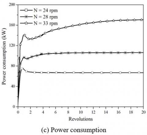
The first object of the simulation is to examine the evolution of the flow structure until the pseudo-steady state is attained. During the calculations, the variation of the volumetric-averaged velocity magnitude in the computational domain, the period-averaged value of the axial flow rate and the moment forces from the surface aerator walls are monitored. Pseudo-steady state condition is assumed when the fluctuations of these variables are low between aerator revolutions. Figure 4 illustrates an example of the numerically calculated values of these variables versus flow time for a submergence depth of +100 mm and three surface aerator speeds, namely 24 rpm, 28 rpm and 32 rpm.
The results of the volumetric-averaged velocity magnitude (Figure 4(a)) show that the volume average velocity increases rapidly during the first revolutions. Thereafter, the volume average velocity gradually reaches a steady state. This feature agrees with numerical observations of Bakker et al. [15]. The number of revolutions to achieve steady state increased from about 12 for N=24 rpm to about 13 for N=28 rpm and 15 for N=30 rpm. Change in time averaged velocity for the simulation time is less than 0.5%.
In Figure 4(b), the period-averaged value of the upward flow rates (wup) versus the axial coordinate, z, is shown for the case at 28 rpm. The upward flow rate is defined as the integral across a section normal to the rotation axis of upward-directed fluxes [16]:
$W_{u p}=\int_{A+} \rho v_Z d A_Z, A^{+}=\left\{d A_Z \in A_Z /v\cdot d A_Z>0\right\}$ (14)
where, v is the velocity, ρ is the density, Azis the section normal to the rotation axis, and A+ is the portion of the section normal to the rotation axis where the axial component of velocity, vz, is directed upward.
The upflow can be used to measure the pumping capacity of the surface aerator and the circulation efficiency of the SAT. At each time, the upflow profile is obtained by calculating the sum of the upward fluxes over sections at different distances from the surface aerator. At first, most of the fluid is at rest, and only the fluid close to the surface aerator blades moves. As the flow develops, reaching the walls of the tank, the fluid streamlines are deflected downward, and the lower regions are gradually driven into motion. The peak corresponds to the upper part of the blades i.e. discharge flux. After 15 surface aerator revolutions, the upflow profile becomes steady and attains pseudo steady state.
Figure 4. Evolution of main flow characteristics used to assess convergence to pseudo-steady state for a submergence depth of +100 mm
Figure 4 (c) shows the evolution of power consumption versus surface aerator revolutions for the three surface aerator speeds. The power consumption is a crucial characteristic of agitated tank and very useful to scale up the results of oxygen transfer rates in SAT. In this study, the power consumption, P, is defined as [17]:
$P=2 \pi N \int_A r \times \Delta P d A$ (15)
where, A is the surface area of the disc and the blades, r is the radial location, Δp is the pressure difference between the front and the back of the surface aerator blades, and dA is the differential surface vector, respectively.
The obtained results show that, the power consumption increases rapidly during the first revolutions and gradually decreases as angular motion is established in the SAT. For high values of the surface aerator rotation speed namely 28 rpm and 33 rpm, when the rotational flow extends out of the surface aerator region (after 1-2 revolutions), the power consumption rises again gradually to reach the steady state condition after about 10 and 16 revolutions of the surface aerator for N=28 rpm and 33 rpm, respectively. This change corresponds to transitions in the structure of the flow field in the SAT. For N=24 rpm, the steady state condition is well established after only 4 revolutions of the surface aerator. Thus, to ensure that the mean quantities given in this study are all obtained from a steady state flow condition, the initial revolutions of the surface aerator are not included in the averaging process and the collection of transient statistics for all the other cases investigated is started only after 15~20 revolutions, depending on the surface aerator speed and submergence depth.
4.1 Validation
To validate the numerical model, the predicted power consumption is averaged over the last 10 s after reaching the steady state condition and the results obtained for different surface aerator rotation speeds are compared to experimental measurements of energy consumption in the literature [18].
As shown in Figure 5, the CFD predicted and the theoretical power consumption profiles are in good agreement, particularly up to 26 rpm where the root-mean-square deviation (RMSD) is less than 5%. For higher values of the surface aerator rotation speed (28 rpm£N£33 rpm), RMS difference increase with the surface aerator rotation, but remain in an acceptable range (<10%), considering the effect of the mesh quality and the experimental uncertainty.
Figure 5. Power consumption as a function of the surface aerator rotation speed: comparison with literature data [18]
To investigate the effect of grid number, various tests are made by changing the discretization step size in the aerator edges and in the axial and radial directions of the tank. The influence of the grid is investigated by demonstrating that the additional cells did not change the RMS deviation of the calculated power consumption by more than 3%. For example, Table 2 reports the calculated power consumption for the different grid size at aerator rotation speeds of 28 rpm and 33 rpm.
Table 2. Examples of grid independence tests
|
Total number of elements |
CFD predicted power consumption P (kW) |
||||
|
28 rpm |
RMSD |
33 rpm |
RMSD |
||
|
Grid 1 |
675458 |
107,24 |
- |
- |
- |
|
Coarsen grid |
882924 |
105,98 |
1,02% |
170,57 |
- |
|
Medium grid |
960037 |
104,73 |
1,01% |
165,65 |
8,51% |
|
Fine grid |
1133136 |
103,48 |
1,01% |
161,97 |
5,22% |
|
Finer grid |
1633136 |
- |
- |
160,05 |
1,88% |
It can be observed that, for N=28 rpm, the increase in grid size is not necessary, comparison leading to almost the same results but with greater computation time. In the case of N=33 rpm, increasing cell numbers from 882924 cells to 960037 cells and then to 1133136 cells change the numerical results remarkably. However, the predicted power consumption tends to be stable after the fine grid (1133136 cells). The coarsen grid is therefore sufficient for low surface aerator rotation speeds, while the fine grid is retained for the surface aerator rotation speeds above 28 rpm to ensure accuracy of the predicted variables. The finest mesh is avoided because it greatly increases the total number of grid elements, requiring the use of significantly lower time steps during the unsteady-state simulations.
4.2 Predicted flow field
Figure 6 shows the predicted pseudo-steady flow field (after 46 s of real time) along the vertical cross section of the SAT and the free surface in terms of normalized magnitude velocity vectors of water for N=24 rpm. The air-water interface is defined as water isosurface with volume fraction equal to 0.9. This value was found in Torré et al. [19] to give the best agreement with experimental data due to the presence of the dynamical equilibrium zone of intense air-water exchanges which occurs around the free surface.
As depicted in Figure 6 (a), the water is drawn from the bottom layer of the SAT into the surface aerator axially, deflected in a radial direction and discharged along the surface aerator with a mean magnitude velocity of up to 2.29. Utip. The discharge profiles developed on the two sides of the surface aerator are clearly different. At the level of the blades (right side of the surface aerator), a partial portion of the propelled water is sprayed into the air and other parts of the flow are discharged into the SAT in the form of a radial jets stream with an upward inclination. However, along the surface aerator disc (left side of the surface aerator) all the propelled water is discharged in the radial direction. If the flow structure in the free surface is considered (Figure 6(b)), a slight deflection of the radial jets stream towards the tangential direction is observed in the surface aerator region due to the centrifugal effects. When these jets strike the unsteady water surface, large water-level fluctuations appears in the surface aerator region. The fluctuations then expand and entrain surrounding water while flowing toward the side wall of the SAT, leading to a significant entrapment of air due to the falling back of the discharged water from the surface aerator blades, and the shearing action at the interface between the fluctuant water and the air [20]. As the distance from the surface aerator increases, the water velocity decreases rapidly and the surface deformation becomes relatively smooth. Upon impingement on the wall, the water flows along the wall vertically downward toward the bottom of the SAT, then the stream returns to the strong upward axial flow below the surface aerator, forming two circulation loops on both sides of the surface aerator. Due to the backflow effect, another small circulation loops appear in the free surface near the SAT walls (Figure 6 (b)), which also leads to air entrainment [20]. Finally, it must be noticed that the flow structure and the velocity distribution of the two developed circulation loops are quite different (Figure 6 (a)). In the right side of the SAT, the center of circulation loop is located in the upper region on the right (y/Y=0.74, z/Z=0.72) with a mean magnitude velocity of 0.032 m. s-1, whereas, in the other side, this structure is observed in center with a slight shift towards the downstream layer (y/Y=-0.51, z/Z=0.7) and a higher mean magnitude velocity. This is explained by the specific design of the Landy-7 surface aerator, especially the odd number of blades (seven blades), that allows the surface aerator to generates simultaneously different effects on its both sides.
4.3 Influence of surface aerator speed
To investigate the effect of surface aerator rotation on the resulting flow in the SAT, contours of normalized velocity with respect to mean magnitude velocity at the yy’ plane and the free surface are presented in Figure 6 for N1=24 rpm and for a higher surface aerator rotation speed (N2=33 rpm). Some streamlines, equally spaced, are added to better understand the fluid direction.
For N1=24 rpm (Figure 7 (a)), the resulting flow appears more uniform with high velocities in the surface aerator region and homogeneous fluid velocity distribution in the remaining parts. These features increase the surface renewal rate at the air-water surface and improve the pollutant removal [21]. However, the dissolved oxygen concentration will then progressively decrease in the SAT especially in the middle zone due to the low lifting capacity of the surface aerator, which allows only small amount of water to flow into the free surface through the surface aerator. By increasing the speed of the surface aerator (N2=33 rpm), the lifting capacity and the intensity of the radial jets of the surface aerator are increased. That results in heterogeneous distribution of the flow velocity in the SAT characterized by an intensive movement along the axial direction and more important radial velocities at the surface aerator region. The interactions of these effects with the swirl motion generated by the rotation of the surface aerator increase turbulence in the SAT and accelerate the exchange of water between the interface layer, which is supersaturated with oxygen, and the shallow layers, leading to a higher oxygen transfer rate and better flow homogenization and dissolved oxygen distribution in the SAT [22].
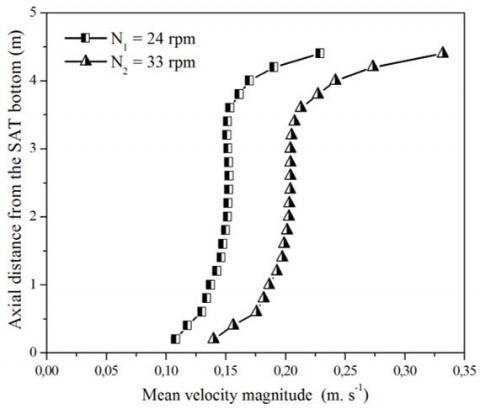
Figure 8 presents the axial distribution of the mean circulation velocity in the SAT for N1=24 rpm and N2=33 rpm.
These results show that the velocity distribution is clearly different for both speeds of the surface aerator. For N1=24 rpm, the flow velocity decreases rapidly with the distance to the surface aerator and reaches constant values of the mean velocity magnitude (v0=0.15 m.s-1) from a depth of 0.9 m to 2.8 m (50% of the total SAT volume). In the remaining part (33% of the total SAT volume), the flow velocity decreases from 0.14 m. s-1 to 0.10 m. s-1. For the higher surface aerator speed (N2=33 rpm), the effect of the flow generated by the rotation of the surface aerator persists longer in the SAT up to a depth of 1.2 m (29% of the total SAT volume), whereas the uniform flow was not observed for a depth greater than 2.2 m. This results in an important bottom part compared to that obtained for the low speed of the surface aerator (43% compared to N1=24 rpm). This difference is explained by the intense lifting capacity of the surface aerator, which accelerates the water flow circulation in the bottom and middle regions, and thus prevents sludge to settle down in these regions and enhance the homogenization of flow in the SAT.
Figure 6. The water flow field for N=24 rpm and submersion depth of +100 mm
Figure 7. Velocity contour at the yy’ plane (left) and the free surface (right)
Figure 8. The mean velocity magnitude along the surface aeration tank depth
Figure 9 shows a quantitative analysis of the proportion of low, medium and high velocities at different surface aerator rotation speeds. The velocity zones are defined as low velocity zone (v<0.025 m. s-1), medium velocity zone (0.025<v<0.3 m. s-1) and high velocity zone (v>0.3 m. s-1), respectively. The three velocity bins are assigned based on the average design velocity, which should be between 0.025 m. s-1 and 0.3 m. s-1 to prevent sludge settling in the SAT [23, 24]. Velocity proportions are presented for the aerator region (z>3 m), the middle zone (1<z<3 m) and the bottom zone of the SAT (z<1 m).
Figure 9. Change in proportions of high, medium and low velocities with the surface aerator rotation speed
The velocity proportions in the aerator region show the aeration efficiency of the Landy-7 surface aerator at low rotation speed, with high velocities in 57% of volume in this region and medium velocities in the remaining volume. By increase the rotational speed of the surface aerator, the proportion of high velocities increased in this region, which improved the rate of oxygen transfer in the upper layers of the SAT.
In the middle region, the low rotational speed achieved medium velocities in nearly 98% of this region, and by increasing the rotational speed of the surface aerator, this proportion decreased to 70% of the volume of the middle region at rotational speed N=33 rpm, whereas the proportion of high velocities only appeared from a rotational speed of 24 rpm and increased with the rotational speed of the surface aerator to 33% of the volume of this region at high rotation speed.
A similar evolution of the proportion of high and medium velocities is observed in the bottom region of the SAT, but with a significant decrease in the proportions of the high velocities (60% compared to the middle region) and slight decreases in the proportion of the medium velocities when the surface aerator rotational speed is greater than 24 rpm. This difference is explained by the decrease in lifting intensity with distance from the Landy-7 surface aerator that allows the low velocities to appear in this region. The increase of the surface aerator ration speed decreases this proportion from 12% to 5% of the volume of the bottom region. It can be noticed that this proportion remains negligible and does not exceed 5% of the total SAT volume, which emphasizes the capacity of the Landy-7 surface aerator to induce turbulence, and thus maintain the sludge in suspension at the lower rotational speed.
The evolution of the proportion of low, medium and high velocities shows the effect of surface aerator rotation speed on aeration and mixing in the SAT. At low rotational speeds, the Landy-7 surface aerator acts as a surface aerator affecting mainly the water near the surface and has little effect on the shallow layers, and at a surface aerator rotational speed higher than 24 rpm this effect appears in the middle, which means that the Landy-7 surface aerator acts as an agitator as well as a surface aerator. It can be noticed that, the presence of these two functions significantly increases the mass transfer capacity of oxygen in the SAT [25].
4.4 Influence of surface aerator submergence depth
The submergence depth of the surface aerator is an important operating parameter in the SAT. Generally, this parameter is described by a dimensionless submergence depth ratio, which is defined as the ratio of the submergence depth of the surface aerator centerline, h, to diameter of the surface aerator, d. In the case of Landy-7 surface aerator, the design specifications require a submergence depth ratio between: h/d=-0.05 and +0.125 (as shown in Figure 1 (b)). To check these requirements, six different submergence depth ratios are studied, including the initial condition, where the surface aerator disc overlaps the initial air-water interface, which corresponds to a submergence depth of 0 m. The other submergence depth ratios studied are: h=-0.05d, +0.031d, +0.063d, +0.094d and +0.125d.
The effect of the submergence depth ratio on the velocity distribution in the SAT is demonstrated in Figure 10, which shows the proportion of low, medium, and high velocities, as well as the mean circulation velocity, at two rotational speeds of the surface aerator, namely N1=20 rpm and N2=33 rpm. The mean circulation velocity is obtained numerically by averaging the magnitude velocity on the entire SAT volume. It can be noticed that the mean circulation velocity can also be predicted using the tracer method [26-28], by introducing a virtual tracer and monitoring the temporal evolution of the mean tracer concentration in the SAT. The distance between two peaks corresponds to the mean circulation time tc from which the mean circulation velocity can be deduced as follows:
$v_0=L / t_c$ (16)
where, L is the length of the flow path.
As can be seen in Figure 10 (a), the proportion of medium velocities first decreases to a minimum value at h/d = 0, and then gradually increases with increasing submergence depth ratio. Accordingly, the air-water interface is determined as the optimum surface aerator position for the lower speed of the surface aerator. It can be noticed that at the optimal submersion ratio, the proportions of high velocities are higher and the zones of low velocities are less than 5% of the total volume of the SAT, which increases the average velocity and thus improves the homogenization in the SAT and reduces the deposition of sludge at the bottom of the tank. At the higher speed, the optimum submergence depth ratio is reached at 0.031, which corresponds to 0.1 m below the initial air-water interface. This difference can be explained by the intense lifting capacity of the Landy-7 surface aerator at high rotational speeds, which keeps the average velocity in the SAT sufficiently high even at large submersion depth ratios.
Figure 10. Change in proportions of high, medium and low velocities with the surface aerator submergence depth ratio
The effect of submersion depth ratio on power consumption is also investigated in this section. As shown in Figure 11, for both surface aerator rotation speeds, the power consumption increases with the submersion depth ratio, and when it reaches the maximum, the power consumption becomes independent of the submersion depth ratio. Finally, it can be seen that the maximum values of power consumption are achieved for submergence depth ratios of 0 and 0.031 which correspond to the optimal submergence depth ratios that were predicted previously for N1=20 rpm and N2=33 rpm, respectively. This indicates that power consumption can be considered as a judgment criterion to determine the optimal surface aerator submergence depth ratio.
Figure 11. Predicted power consumption as a function of the surface aerator submergence depth ratio
The flow field is investigated in a full-scale SAT equipped with a Landy-7 surface aerator using a coupled VOF k-ε turbulence model and the MRF method, implemented in the commercial CFD code FLUENT. Simulations are performed for different rotational speeds and submergence depth ratios of the landy-7 surface aerator until the pseudo-steady flow field is attained, and predictions are analyzed and compared by considering two important factors: flow field and power consumption. The following conclusions are obtained:
The fully developed flow field in the SAT is achieved after 15 to 20 revolutions, depending on the surface aerator speed and submergence depth.
CFD calculations picked up the hydrodynamic characteristics of the flow field in the SAT, and predicted power consumption at different rotational speeds are in significant agreement with the experimental data available in the literature. Thus, the present CFD model can be a valuable tool to improve the hydrodynamic performance of the SAT.
The detailed analysis of flow revealed a complex behavior, consisting of two different circulation loops on both sides of the surface aerator, with high velocities in the surface aerator region and a homogeneous fluid velocity distribution in the remaining parts. This implies that the landy-7 surface aerator acts as a surface aerator and its effects are mainly limited to the surface layers. At higher rotational speeds, the flow generated by the surface aerator extended into the deeper layers and the regions of low velocities decreased, which indicates the effectiveness of the Landy-7 surface aerator to provide both aeration and mixing.
The combination of proportions of high, medium and low velocities and power consumption showed that the air-water interface is the optimal surface aerator location for the low surface aerator speed. This location of the surface aerator can improve homogenization in the SAT and prevent sludge deposition at the bottom of the SAT. At higher rotational speed, the optimal surface aerator submergence depth ratio is 0.031, which corresponds to 0.1 m below the initial air-water interface.
This study is the first step to disclose the hydrodynamic characteristics of the SAT. Further numerical analysis for multiphase flow and quantitative comparison with experimental results are required to extend the validity of present results. In addition, the results of this research provide useful guidance for practitioners to improve the performance of SAT by adjusting the operating conditions namely aerator rotation speed and submergence depth according to the desired operation, i.e. aeration or both aeration and agitation.
|
d |
Surface aerator diameter, m |
|
g |
gravitational acceleration, m. s-2 |
|
h |
Surface aerator submergence depth, m |
|
h/d |
Submergence depth ratio |
|
h0 |
Water depth, m |
|
k |
Turbulent kinetic energy, m2 s -2 |
|
N |
Surface aerator rotation speed, rpm |
|
P |
Power consumption, kW |
|
p0 |
Reference pressure, Pa |
|
$\mathrm{U}_{\mathrm{tip}}$ |
velocity at the tip of the aerator, (m s-1) |
|
v |
Fluid velocity, m. s-1 |
|
$v_0$ |
Mean circulation velocity, (m. s-1) |
|
w |
Inner tank width, m |
|
$\mathrm{w}_{\text {up }}$ |
Upward flow rate, m3. s-1 |
|
z |
Axial distance from the SAT bottom, m |
|
Greek symbols |
|
|
$\Delta t$ |
Time step, s |
|
$\alpha_c$, $\alpha_d$ |
Volume fraction |
|
ε |
Turbulent dissipation rate, m2 .s-2 |
|
$\mu_c$,$\mu_d$ |
Dynamic viscosity, kg. m-1.s-1 |
|
$\rho_c$,$\rho_d$ |
Density, kg. m-3 |
|
σ |
Surface tension coefficient, N. m–1 |
|
Subscripts |
|
|
c |
Continuous phase |
|
d |
Discrete phase |
|
Abbreviation |
|
|
VOF |
Volume Of Fluid method |
|
CFD |
Computational Fluid Dynamics |
|
CSF |
Continuum Surface Force |
|
MRF |
Multiple Reference Frame approach |
|
RANS |
Reynolds-Averaged Navier-Stokes |
|
RMSD |
Root-Mean-Square Deviation |
|
SAT |
Surface Aeration Tank |
|
SIMPLE |
Semi-Implicit Pressure Method for Pressure Linked Equations |
|
SM |
Sliding Mesh model |
|
WWTP |
Wastewater Treatment Plant |
[1] Banaei, F.K., Zinatizadeh, A.A.L., Mesgar, M., Salari, Z., Sumathi, S. (2013). Effect of biomass concentration and aeration rate on performance of a full-scale industrial estate wastewater treatment plant. Journal of Environmental Chemical Engineering, 1(4): 1144-1153. https://doi.org/10.1016/j.jece.2013.08.033
[2] Zamouche, R., Bencheikh-Lehocine, M., Meniai, A.H. (2007). Oxygen transfer and energy savings in a pilot-scale batch reactor for domestic wastewater treatment. Desalination, 206: 414-423. https://doi.org/10.1016/j.desal.2006.03.576
[3] Zlokarnik, M. (1979). Scale-up of surface aerators for waste water treatment. Advances in Biochemical Engineering, 11: 157-180. https://doi.org/10.1007/3-540-08990-X_25
[4] Backhurst, J.R., Harker, J.H., Kaul, S.N. (1988). The performance of pilot and full-scale vertical shaft aerators. Water Research, 22(10): 1239-1243. https://doi.org/10.1016/0043-1354(88)90110-8
[5] Patil, S.S., Deshmukh, N.A., Joshi, J.B. (2004). Mass-transfer characteristics of surface aerators and gas-inducing impellers. Industrial & Engineering Chemistry Research, 43(11): 2765-2774. https://doi.org/10.1021/ie030428h
[6] Wei, W., Liu, Y., Lv, B. (2016). Numerical simulation of optimal submergence depth of impellers in an oxidation ditch. Desalination and Water Treatment, 57(18): 8228-8235. https://doi.org/10.1080/19443994.2015.1021840
[7] Deshmukh, N.A., Joshi, J.B. (2006). Surface aerators. Chemical Engineering Research and Design, 84(11): 977-992. https://doi.org/10.1205/cherd05066
[8] Rao, A.R., Patel, A.K., Kumar, B. (2010). Power characteristics of surface aerators. Journal of Chemical Technology & Biotechnology, 85(6): 805-813. https://doi.org/10.1002/jctb.2364
[9] Stamou, A.I. (1993). Prediction of hydrodynamic characteristics of oxidation ditches using the k-ε turbulence model. In Engineering Turbulence Modelling and Experiments, 261-270. https://doi.org/10.1016/B978-0-444-89802-9.50029-0
[10] Kang, Q., He, D., Zhao, N., Feng, X., Wang, J. (2020). Hydrodynamics in unbaffled liquid-solid stirred tanks with free surface studied by DEM-VOF method. Chemical Engineering Journal, 386: 122846. https://doi.org/10.1016/j.cej.2019.122846
[11] Huang, W., Li, K., Wang, G., Wang, Y. (2013). Computational fluid dynamics simulation of flows in an oxidation ditch driven by a new surface aerator. Environmental Engineering Science, 30(11): 663-671. https://doi.org/10.1089/ees.2012.0313
[12] Brackbill, J.U., Kothe, D.B., Zemach, C. (1992). A continuum method for modeling surface tension. Journal of Computational Physics, 100(2): 335-354. https://doi.org/10.1016/0021-9991(92)90240-Y
[13] Yang, Y., Yang, J., Zuo, J., Li, Y., He, S., Yang, X., Zhang, K. (2011). Study on two operating conditions of a full-scale oxidation ditch for optimization of energy consumption and effluent quality by using CFD model. Water Research, 45(11): 3439-3452. https://doi.org/10.1016/j.watres.2011.04.007
[14] Launder, B.E., Spalding, D.B. (1974). The numerical computation of turbulent flows. Computer Methods in Applied Mechanics and Engineering, 3(2): 269-289. https://doi.org/10.1016/0045-7825(74)90029-2
[15] Bakker, A., Oshinowo, L.M. (2004). Modelling of turbulence in stirred vessels using large eddy simulation. Chemical Engineering Research and Design, 82(9): 1169-1178. https://doi.org/10.1205/cerd.82.9.1169.44153
[16] Campolo, M., Paglianti, A., Soldati, A. (2002). Fluid dynamic efficiency and scale-up of a retreated blade impeller CSTR. Industrial & Engineering Chemistry Research, 41(2): 164-172. https://doi.org/10.1021/ie010225y
[17] Taghavi, M., Zadghaffari, R., Moghaddas, J., Moghaddas, Y. (2011). Experimental and CFD investigation of power consumption in a dual Rushton turbine stirred tank. Chemical Engineering Research and Design, 89(3): 280-290. https://doi.org/10.1016/j.cherd.2010.07.006
[18] Landy-7 Surface Aerator User's Manual. https://www.westech-inc.com/products/surface-aerator-landy-7, accessed on 29 June 2022.
[19] Torré, J.P., Fletcher, D.F., Lasuye, T., Xuereb, C. (2007). An experimental and computational study of the vortex shape in a partially baffled agitated vessel. Chemical Engineering Science, 62(7): 1915-1926. https://doi.org/10.1016/j.ces.2006.12.020
[20] Luo, P., Wu, J., Pan, X., Zhang, Y., Wu, H. (2016). Gas-liquid mass transfer behavior in a surface-aerated vessel stirred by a novel long-short blades agitator. AIChE Journal, 62(4): 1322-1330. https://doi.org/10.1002/aic.15104
[21] Simon, S., Roustan, M., Audic, J.M., Chatellier, P. (2001). Prediction of mean circulation velocity in oxidation ditch. Environmental Technology, 22(2): 195-204. https://doi.org/10.1080/09593332208618295
[22] Matko, T., Chew, J., Wenk, J., Chang, J., Hofman, J. (2021). Computational fluid dynamics simulation of two-phase flow and dissolved oxygen in a wastewater treatment oxidation ditch. Process Safety and Environmental Protection, 145: 340-353. https://doi.org/10.1016/j.psep.2020.08.017
[23] Raschid-Sally, L., Roustan, M., Roques, H., Faup, G.M. (1987). Study of a non-conventional aeration system. Water Science and Technology, 19(5-6): 869-876. https://doi.org/10.2166/wst.1987.0265
[24] Bridgeman, J. (2012). Computational fluid dynamics modelling of sewage sludge mixing in an anaerobic digester. Advances in Engineering Software, 44(1): 54-62. https://doi.org/0.1016/j.advengsoft.2011.05.037
[25] Roustan, M., Chatellier, P., Lefevre, F., Audic, J.M., Burvingt, F. (1993). Separation of the two functions aeration and mixing in oxidation ditches: Application to the denitrification by activated sludge. Environmental Technology, 14(9): 841-849. https://doi.org/10.1080/09593339309385356
[26] Bekrentchir, K., Debab, A. (2016). Numerical investigation of mixing time in a torus reactor. Periodica Polytechnica Chemical Engineering, 60(3): 210-217. https://doi.org/10.3311/PPch.8637
[27] Zaheri, K., Bayareh, M., Nadooshan, A.A. (2019). Numerical simulation of the motion of solid particles in a stirred tank. International Journal of Heat and Technology, 37(1): 109-116. https://doi.org/10.18280/ijht.370113
[28] Zhang, J., Pierre, K.C., Tejada-Martinez, A.E. (2019). Impacts of flow and tracer release unsteadiness on tracer analysis of water and wastewater treatment facilities. Journal of Hydraulic Engineering, 145(4): 1-11. https://doi.org/10.1061/(ASCE)HY.1943-7900.0001569