Kaustubh G. Kulkarni* | Sanjay N. Havaldar | Harsh V. Malapur
© 2022 IIETA. This article is published by IIETA and is licensed under the CC BY 4.0 license (http://creativecommons.org/licenses/by/4.0/).
OPEN ACCESS
Concentrated solar power (CSP) is a cutting-edge method of conserving renewable energy. The concentrated solar power is utilized as a heating source to increase the temperature of heat transfer fluid circulating in the piping of the central solar receiver. The solar central receiver is the most crucial part in solar tower power plants. In this study, a Computational Fluid Dynamics (CFD) framework was developed for analyzing four designs of the central tower receiver, namely, a conventional uniform tube diameter solar receiver (UTD), vertical variable tube diameter solar receiver (VTD), a circular solar variable tube diameter (CVTD) receiver and a leaf type circular solar receiver (LTSR). This analysis studied the solar radiation heat transfer efficiency, temperature distribution, and fluid outlet temperature; pressure and velocity distributions for the designs using CFD. It was found that the CVTD design helped achieve a higher rise in temperature of the heat transfer fluid (HTF) when the mass flow rate was in the range of 0.1 to 0.2 liter per minute. The CVTD and LSTR models of receiver were more efficient heat transfer receiver designs compared with other designs for same surface area and strength of beam radiations.
CFD, heliostats, solar energy concentrator, leaf type solar receiver, vertical variable tube receiver
Solar energy is the driving force behind all of the civilization on earth. Natural processes and geomorphological modifications aided the evolution of conventional energy sources on earth since millions of years [1]. Despite the fact that traditional energy resources have such a higher power density, the availability of technical support and the simplicity with which they can be used pollutes the environment by emitting toxic gases and radiations [2]. Solar energy is a relatively clean source of energy [3] and is now the most dependable alternative energy source. It could not be directly utilized to generate power because of its lower intensity [4]. This dilute source could be utilized for a broad range of input systems, from domestic to industrial, by creating proper concentrating arrangements [5]. Intense sunlight irradiates absorber tubes in compact solar thermal power plants with a centralized receiver, converting solar power into heat. The heat flux density on a densely packed surface may extend up to 2.5 MW/m2. The heat flux density distribution on the receiver surface is usually determined by the aiming method [6].
Solar thermochemical processes frequently necessitate high temperatures, which could be obtained through direct solar energy absorption. The concentrated solar energy is transported from the tube walls of the receiver to the heat transfer fluid that goes along a heat exchanger for producing steam for the Rankine cycle in a traditional central receiver system [7]. As a result, a higher working fluid temperature is linked to increased receiver and power cycle efficiency [8]. Solar energy could be transformed directly into electricity using photovoltaic systems, which could then be saved in batteries for later usage. Solar systems that capture solar energy and transmit through the working fluid in the form of sensible heating of the fluid that constantly flows via tubes are another form of the solar system [9]. Solar receivers are heat exchangers that transfer solar energy to heat energy through the use of water. Then the fluid transfers the thermal energy to steam that will then be passed through a turbine to generate electricity [10].
Solar radiations are a high-temperature, high-energy source of an irradiation of roughly 63 MW/m2 [11]. These radiations are utilized as thermal energy when they are directed on a receiver or concentrating device [11]. Several authors have looked into incorporating solar thermal power into high-temperature production processes, using Computational Fluid Dynamics (CFD) to analyze high- temperature solar devices for improving prototype designs and the high-temperature process' performance [12]. The solar prototype was made up of 3 layers of material (refractory, frame and insulation) and also was designed to attain the maximum temperature range with more uniform thermal profile [13]. As a result, the CFD model produced was used to investigate the thermal behavior of various prototype configurations. Different configurations and refractory materials with varied thicknesses are used for the prototype model [14].
The goal of this research is to evaluate receiver simulation using sophisticated CFD systems, as well as conduct an empirical examination on the circular receiver for various mass flow rates and heat transfer rates using water [15]. The amount of solar irradiations reflected by the heliostats on the receiver determines the amount of heat input to the receiver [16]. An analytical framework that could be employed for 'n' no. of mirrors was utilized for selecting a tiny central receiver system and an empirical investigation of temperature readings of working fluid in a spiral receiver was performed for variable heat flux and mass flow rate [17]. In addition, the CFD results for a circular solar receiver are compared with a conventional solar receiver for the pressure drop and heat transfer coefficient [18]. The simulation is based on the realistic heat flux distributions considered as an advantage on the surface of receiver. CFD simulations and measurements are performed using the FORTAN code [19]. Solar cavity receiver based on CFD analysis performed with respect to air flow and through 10 KW HFSS-High Flux Solar Simulator it has been irradiated directly [20]. This paper discusses the analytical model, experimental test setup, CFD analysis, and findings for three different models of central solar receiver using Ansys®2016.
The solar receiver receives reflected solar irradiations from a number of heliostats (reflective mirrors) in a concentrated solar power (CSP) plant. The sun tracking system uses a solar sensor mounted on the heliostat supporting structure to track the sun such that the heliostat inside the surface always reflects the solar irradiations onto the central receiver (placed centrally on a tower). The central receiver receives concentrated beam radiations. It is generally made of copper with refractory liners and absorber coating and acts as a heat exchanger. Figure 1 shows the schematic of a CST power generation plant concept.
Figure 1. A typical layout of a solar power plant (CST) with receiver
Figure 2. A layout of numerical modeling and simulation
A typical layout for the receiver numerical modeling and simulation is as shown in Figure 2. The fluid enter all the solar receiver models being analyzed from the bottom header and leaves from the top header. As solar rays are directed towards the receiver, the concentrated beam irradiation varies from the point of concentration (usually the center of receiver) to its periphery. The solar beam received on the receiver has an irradiance distribution as shown in Figure 3 [3]. In Figure 3, the solar beam irradiation profile of the concentrated beam radiations on the receiver placed atop the tower is shown. The irradiance has a higher value of flux at the center and dilute at the edges.
Figure 3. Irradiance distribution map of the solar beam received by the receiver surface [3]
3.1 Physical models
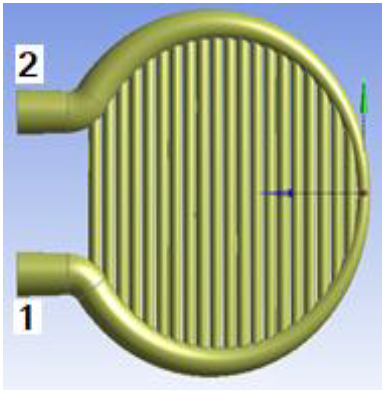
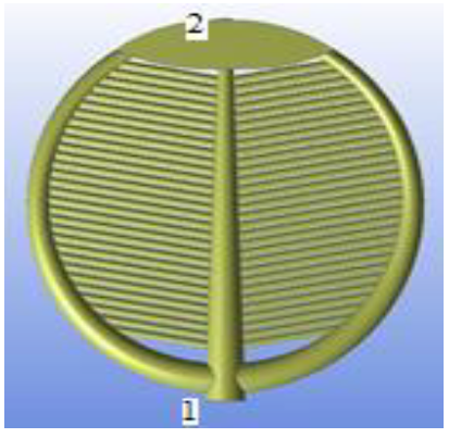
Four types of receivers were modeled for numerical simulation and comparison which are as shown in Figures 4(a) to 4(d). The simplest of ideas is the constant diameter billboard receiver is as shown in Figure 4(a). The cold heat transfer fluid (HTF) enter from the bottom header and hot HTF leaves from the billboard receiver from the top header. As the concentrated solar beam temperature intensity is greater at the center than at its circumference, a vertical variable header variable tube diameter receiver was modelled which is as shown in Figure 4(b). In this model (Figure 4(b)) the cold HTF enter centrally from the bottom header and hot HTF leaves from the receiver centrally from the top header. In the third type of model, the receiver was modeled of a circular variable diameter header (Figure 4(c)). In Figure 4(d), a leaf type circular solar receiver model is presented. In this model, the HTF enter from the bottom header (from the center), the header is of varying diameter from bottom to top. The receiver tubes are inclined to help hot HTF to move upwards (by density difference once heated). The hot HTF gets collected in the top chamber and can be used for heating in a heat exchanger further in the process. The leaf type center solar receiver (Figure 4(d)) is modeled for attaining a suitably higher mean temperature after mixing of the HTF from all the branches of the inclined tubes of the receiver.
The four receiver modelled in Figure 4 had approximately same surface area of 0.6 m2. The beam flux concentrated on the modelled receivers was varied from 1000 to 3000 W/m2 and the mass flow rate was varied from 0.1 litres per minute (LPM) to 0.5 LPM in steps of 0.1 LPM in the analysis of all the models. Various other parameters used for modelling and in the CFD analysis are in Table 1.
|
(a) UTD |
(b) VTD |
(c) CVTD |
(d) LTSR |
Figure 4. Various models of solar receivers in the simulation with 1 and 2 are input and output respectively
Table 1. Design dimensions and materials in the simulation
|
No |
Parameters |
|
|
1 |
Diameter of the bottom header inlet and outlet (mm) |
50 and 15 |
|
2 |
Diameter of the upper header inlet and outlet (mm) |
15 and 50 |
|
3 |
Area of the receiver (m2) |
0.6 |
|
4 |
Tube Thickness (mm) |
1 |
|
5 |
Mass Flow Rate (LPM) |
0.1 |
|
6 |
Heat Flux (w/m2) |
1000 to 3000 |
|
7 |
Material of Receiver |
Copper |
3.2 Mathematical model
The central receiver absorbs the sun energy concentrated on it and transmits the heat absorbed to the working fluid (HTF). Tubes with excellent thermal conductivity and durability are used for high effectiveness and thermal efficiency. The availability of heat flux is high in the central inner region and low in the outside region (refer to Figure 3). The heat flow zone with the highest heat flux is in the center of the receiver, whereas the heat flux zone with the lowest heat flux is on the outside. As a result, utilizing a circular design for the receiver and lead tube design was investigated over conventional straight tube design. Therefore, the mathematical modelling of a receiver is explained as below:
The receiver tube's length of the available focus area is represented as,
$L=\pi * \frac{D_{0}+D_{1}}{2}$ (1)
Eq. (1) was multiplied by $\pi$ to obtain L in the circular case.
For the accessible mirror area, the theoretical heat rate on the circular receiver can be given as,
$Q=I_{B} \gamma_{b} \rho A_{m}$ (2)
The beam radiation is obtained using:
$\mathrm{I}_{B}=I_{G}-I_{D}$ (3)
The energy balance for a receiver can be written as follows:
$Q_{t}=Q_{a}+Q_{c}+Q_{\gamma}$ (4)
For copper receiver, the density considered was 8978 kg/m3, Cp assumed was 381 J/kg-K with thermal conductivity as 387 W/m-K. The absorbity fraction that was used in the anlysis softwas was 0.8, thus reflectivity was 0.2. That is out of the total Qt in Eq. (4), Qa (absorbivity) was 80%, Qc is due to material copper and Qy (reflectivity) was 20% respectively.
Heat transfer coefficient due to convective losses
$h=5.7+3.8 \mathrm{~V}$ (5)
The temperature of the working fluid at the outlet was determined by,
$\frac{I_{b} \gamma_{b} \rho \alpha A_{m}-h \cdot A_{0}\left(T_{w}-T_{a}\right)-\varepsilon \cdot A_{0} K_{b}\left(T_{\omega}^{4}-T_{a}^{4}\right)}{m c_{p}}+T_{i}=T_{0}$ (6)
If Q is the solar flux input / solar irradiation then the heat absorbed by HTF was obtained (the product of mass flow rate of HTF in kg/s, specific heat capacity of water in J/kg.K, and temperature gain). The efficiency (ƞ) was the ratio of heat absorbed by HTF to the solar flux input.
3.3 Numerical modelling
A numerical analysis for the modelled solar receivers was performed using ANSYS®16. The models follow the following equations for continuity, momentum and energy.
The continuity equation,
$\frac{\partial u_{i}}{\partial x_{i}}=0$ (7)
The momentum equation,
$\frac{\partial u_{i} u_{j}}{\partial x_{i}}=-\frac{1}{\rho} \frac{\partial p}{\partial x_{i}}+\frac{\partial}{\partial x_{i}}\left(\left(v+v_{t}\right)\left(\frac{\partial u_{i}}{\partial x_{j}}+\frac{\partial u_{j}}{\partial x_{i}}\right)\right)$ (8)
The energy equation,
$\frac{\partial u_{i} T}{\partial x_{i}}=\rho \frac{\partial}{\partial x_{i}}\left(\left(\frac{v}{P_{r}}+\frac{v_{t}}{P_{r}}\right) \frac{\partial T}{\partial x_{i}}\right)$ (9)
The domain definitions and boundary conditions for numerical simulations are as shown in Table 2. SIMPLE algorithm was used with finite-volume formulation to solved for convergence in the simulation. A standard scheme was used for the pressure term and the first-order upwind scheme was adopted for the governing equations.
Ansys 2016 was used to simulate the results. The output from the software was recorded and analyzed. Various settings used in the simulation are in Table 4.
Table 2. Boundary conditions settings
|
Boundary conditions |
|
|
Inlet |
Mass flow-Inlet |
|
Outlet |
pressure-Outlet |
|
Initial pressure (gauge) |
zero Pascal |
|
Temperature (inlet) |
300 K |
Table 3. Values of parameters in the simulation
|
Parameter |
Value |
|
Density of water (kg/m3) |
998.2 |
|
The mass flow rate (kg/s) |
Varied |
|
The volumetric flow rate (LPM) |
Varied |
|
Density of Copper (kg/m3) |
8960 |
|
Specific Heat of Copper (J/kg-K) |
385 |
|
Solar Simulator Irradiation (W/m2) |
Varied |
Table 4. Settings for ANSYS simulation
|
Parameter |
Setting |
|
Working fluid |
Water |
|
Pipe material |
Copper |
|
Model used |
Energy |
|
Pressure Velocity Coupling Scheme |
SIMPLE |
|
Spatial Gradient |
Green Gauss Cell Based |
|
Initialization |
Standard |
|
No. of Iterations |
30 |
|
Computed for |
All zones |
The effectiveness of the conventional solar receiver is evaluated using temperature, pressure and velocity measure. The CFD output for the variation of HTF temperature, pressure and velocity for the modeled UTD solar receiver is presented in Figures 5 to 7 respectively. It is observed from Figure 5 that the HTF temperature had a peak value at the right-top zone of receive tubes and header for the UTD model. A lower HTF temperature zone was observed at the entry of header for the UTD model. The central zone of the UTD showed an average temperature level for the HTF. The pressure variation (refer to Figure 6) of the HTF for the UTD suggest that there is lower pressure at the upper left exit zone (as seen by the blue shade) while there is a higher pressure developed at the far end on the right side tubes (as indicated by the red shade). The cold HTF entered the intake via the bottom-left header, and the flow attempted to follow the shortest path to the output header (top header). This phenomenon occurs continuously, thereby the blue color area is always at a reduced temperature distribution. The mass flow rate of HTF on the far sides of the tube is reduced, thus the yellow and red color shows that the temperature from irradiation is not utilized on the right-top side of the receiver. There is no or little mass of HTF that flows further down through the tubes of the UTD receiver model.
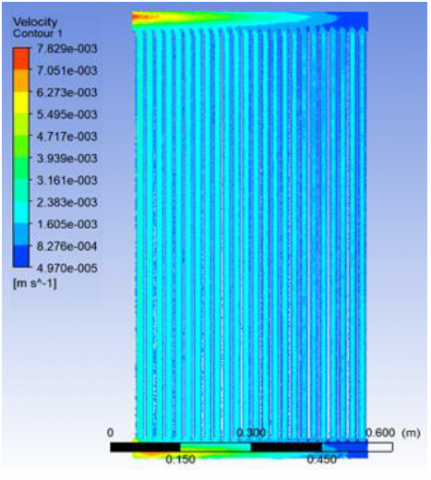
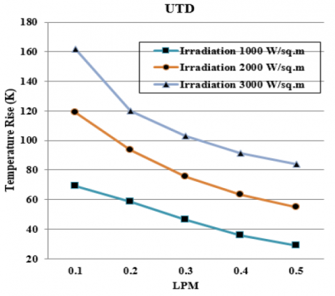
In Figure 6 it is observed that the fluid (HTF) pressure was higher from the bottom-left upwards. The pressure of HTF at the far-right top portion of the tubes consequently is low as is observed from the simulation output in Figure 6. The pressure variation is inversely indicated in the CFD out of the HTF variation of velocity in the UTD as observed in Figure 7. Figure 8 is a plot of temperature difference (To – Ti) of the HTF versus mass flow rate in liter per minute (LPM) using UTD model in the simulation. From Figure 8, it can be seen that for a lower mass flow of HTF in the UTD, the value temperature difference (To – Ti) is higher. This suggests that the time required to absorb heat from the beam solar radiation incident on the UTD surface must be higher to obtain a higher (To – Ti).
Figure 5. Variation of HTF temperature in the UTD
Figure 6. Variation of HTF pressure in the UTD
Figure 7. Variation of HTF velocity in the UTD
Figure 8. HTF Temperature rise versus flow rate for UTD
Figure 9. Variation of HTF temperature in the VTD
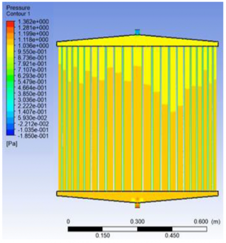
Figure 10. Variation of HTF pressure in the VTD
The CFD output for the variation of HTF temperature, pressure, velocity and the plot of variation of (To – Ti) with mass flow rate in LPM for the modeled VTD solar receiver is presented in Figures 9 to 12 respectively. A lower HTF temperature zone was observed at the central tubes of the VTD model. The pressure variation (refer to Figure 10) of the HTF for the VTD suggest that there is a higher pressure at the upper section (as seen by the yellow shade) while there is a lower pressure developed at the lower receiver zone (as indicated by the green shade). Various values of parameter assumed for the CFD simulation (Tables 3 and 4). As cold HTF entered the intake from the bottom centre header, the flow tried to take the shortest route to the exit header (top header) through the centre larger diameter tubes. This phenomenon occurs continuously, thereby the blue color area is always at a reduced temperature distribution that is seen in the center zone of VTD. This suggests that the mass flow rate is higher in the centrer tubes thus absorbing lower solar radiations that are incident on the VTD (refer to Figure 9).
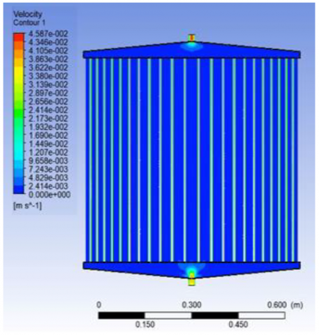
Figure 11. Variation of HTF velocity in the VTD
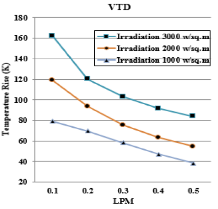
Figure 12. HTF Temperature rise versus flow rate for VTD
The CFD analysis output for the variation of HTF temperature, pressure, velocity and the plot of variation of (To – Ti) with the mass flow rate in LPM for the modeled CVTD solar receiver is presented in Figures 13 to 16 respectively. Figure 13 shows the temperature variation for modelled CVTD. In Figure 13, it was observed that due to the centrifugal force in the circular region, the temperature distribution varies. It is noticed that at the curved section, tube experiences higher centrifugal force thus causes high temperature at the tube’s curved section and less temperature at the entry of cold HTF in the tube. Figure 14 shows the map of the variation of velocity in the modelled CVTD. The velocity distribution is low in the curved portion due to the lower centrifugal force, and the velocity dispersion is enhanced due to the larger centrifugal force at the HTF entry into the CVTD, as shown in Figure 14. header (top header) by the closest route in the central greater diameter tubes. This phenomenon occurs continuously, thereby the blue color area is always at a reduced temperature
Figure 16 is a plot of temperature difference (To – Ti) of the HTF versus mass flow rate in liter per minute (LPM) using CVTD model in the simulation.
Figure 13. Variation of HTF temperature in the CVTD
Figure 14. Variation of HTF pressure in the CVTD
Figure 15. Variation of HTF velocity in the CVTD
Figure 16. HTF temperature rise versus flow rate for CVTD
From Figure 16, it is observed that for lower mass flow of HTF in the CVTD model, the value temperature difference (To – Ti) is higher than the temperature difference (To – Ti) in the UTD and VTD model. This suggests that the absorption of heat from the beam solar radiations incident on the CVTD is utilized as HTF is exposed to concentrate solar radiation in the central portion where the temperature profile has higher heat flux (refer to Figure 3).
Figure 17. Variation of HTF temperature in the LTSR
Figure 18. Variation of HTF pressure in the LTSR
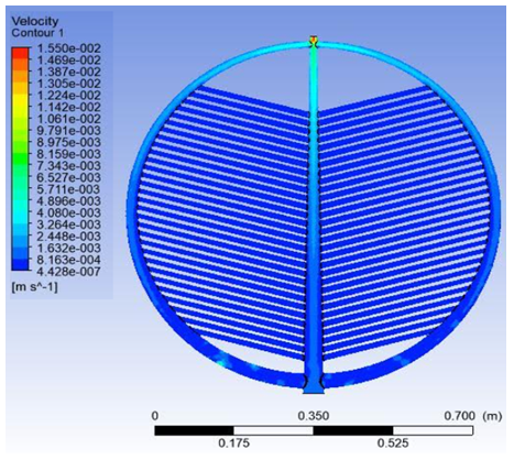
Figure 19. Variation of HTF velocity in the LTSR
The CFD analysis output for the variation of HTF temperature, pressure, velocity and the plot of variation of (To – Ti) with mass flow rate in LPM for the LTSR model is presented in Figures 17 to 20 respectively. Figure 17 shows the temperature variation for modelled LTSR. In Figure 17, it was observed that due to the in the circular region, the temperature distribution varies. It is noticed that at the curved section, tube experiences higher centrifugal force thus causes high temperature at the tube’s curved section and less temperature at the entry of cold HTF in the tube. Figure 18 shows the map of the variation of velocity in the modelled LTSR. The velocity distribution is low in the curved portion due to the lower centrifugal force, and the velocity dispersion is enhanced due to the larger centrifugal force at the HTF entry into the CVTD, as shown in Figure 18.
Figure 20. HTF temperature rise versus flow rate for LTSR
Figure 21. Variation of HTF temperature difference (To – Ti) versus HTF flow rate in LPM in receivers at 3000 W/m2 solar intensity
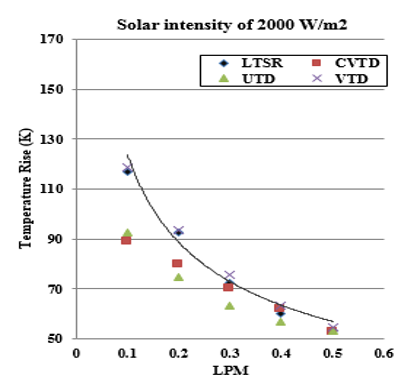
Figure 22. Variation of HTF temperature difference (To – Ti) versus HTF flow rate in LPM in receivers at 2000 W/m2 solar intensity
Figures 21 to 23 are the comparison of the rise in temperature, (To – Ti) of HTF (the initial temperature was set to 300 K) for irradiation solar intensity of 3000, 2000 and 1000 W/m2. It was found that the VTD model for the receiver has a greater temperature rise for the HTF as the mass flow rate was varied in the analysis. Secondly, it can also be observed that for low mass flow rates (0.1 and 0.2 LPM) the temperature gained by the HTF was higher. This was because the HTF flows with a lower velocity in receiver tubes and stays for a longer time in the tube. Thus, the HTF absorbs more heat from the irradiations at lower mass flow rates.
Figure 23. Variation of HTF temperature difference (To – Ti) versus HTF flow rate in LPM in receivers at 1000 W/m2 solar intensity
In this numerical analysis, the temperature, velocity and pressure distribution of HTF (water) for four different solar receiver geometries were analysed using Ansys®2016.
The intensity of solar beam was varied and the flow rate of HTF was varied. The solar receiver surface area in all the four modelled receivers was approximately constant. The heat absorbed by the HTF (To – Ti) in the variable tube diameter (VTD) receiver model was found to be higher than in all other models studied. For lower mass flow rate, the velocity of HTF being low, heat absorbed by the HTF is higher than higher mass flow rates in the receiver.
We thank Dr. Vishwanath Karad MIT World Peace University, Pune for allowing us to use their CFD simulation software for this analysis.
|
Do |
outside diameter of the tube |
|
Di |
inside diameter of the tube |
|
L |
length of the tube |
|
Q |
theoretical heat rate |
|
Am |
mirror area (m2) |
|
IB |
solar beam radiation (w/m2) |
|
IG |
global radiation (w/m2) |
|
ID |
diffuse radiation (w/m2) |
|
Qt |
heat absorbed by receiver (W) |
|
Qa |
heat absorbed by working fluid (W) |
|
Qc |
convective losses (W) |
|
Qγ |
radiation loses (W) |
|
h |
heat transfer coefficient (w/m2 K) |
|
A0 |
the receiver absorber area (m2), |
|
Ta |
the Ambient temperature of air (K) |
|
Tw |
mean temperature of tube surface (K) |
|
T0 |
is the outlet temperature of working fluid (K) |
|
Ti |
the Inlet temperature of working fluid (K) |
|
m |
mass flow rate (Kg/sec) |
|
cp |
specific heat (kJ/Kg k) |
|
Greek symbols |
|
|
ρ |
reflectivity of mirror |
|
ε |
the emissivity of tube material |
|
Subscripts |
|
|
i |
Outside or outer |
|
o |
Insider or inner |
|
1 |
HTF inlet |
|
2 |
HTF outlet |
[1] Verma, S.K., Sharma, K., Gupta, N.K., Soni, P., Upadhyay, N. (2020). Performance comparison of innovative spiral shaped solar collector design with conventional flat plate solar collector. Energy, 194: 116853. https://doi.org/10.1016/j.energy.2019.116853
[2] Fritsch, A., Uhlig, R., Marocco, L., Frantz, C., Flesch, R., Hoffschmidt, B. (2017). A comparison between transient CFD & FEM simulations of solar central receiver tubes using molten salt and liquid metals. Solar Energy, 155: 259-266. https://doi.org/10.1016/j.solener.2017.06.022
[3] Boerema, N., Morrison, G., Taylor, R., Rosengarten, G. (2013). High temperature solar thermal central-receiver billboard design. Solar Energy, 97: 356-368. https://doi.org/10.1016/j.solener.2013.09.008
[4] Abuseada, M., Ozalp, N. (2020). Experimental and numerical study on a novel energy efficient variable aperture mechanism for a solar receiver. Solar Energy, 197: 396-410. https://doi.org/10.1016/j.solener.2020.01.020
[5] Ophoff, C., Abuseada, M., Ozalp, N., Moens, D. (2020). Systematic approach for design optimization of a 3 KW solar cavity receiver via multiphysics analysis. Solar Energy, 206: 420-435. https://doi.org/10.1016/j.solener.2020.06.021
[6] Vignarooban, K., Xu, X.H., Arvay, A., Hsu, K., Kannan, A.M. (2015). Heat transfer fluids for concentrating solar power systems – a review. Applied Energy, 146: 383-396. https://doi.org/10.1016/j.apenergy.2015.01.125
[7] Ozalp, N., JayaKrishna, D. (2010). CFD analysis on the influence of helical carving in a vortex flow solar reactor. Int J Hydrog Energy, 35(12): 6248e60. https://doi.org/10.1016/j.ijhydene.2010.03.100
[8] Rodat, S., Abanades, S., Sans, J.L., Flamant, G. (2009). Hydrogen production from solar thermal dissociation of natural gas: development of a 10 kW solar chemical reactor prototype. Sol Energy, 83: 1599e610.
[9] Z'Graggen, A., Steinfeld, A. (2009). Heat and mass transfer analysis of suspension of reacting particles subjected to concentrated solar radiation-Application to the steam-gasification of carbonaceous materials. Int J Heat Mass Trans., 52(1-2): 385-395. https://doi.org/10.1016/j.ijheatmasstransfer.2008.05.023
[10] Jamel, M.S., Rahman, A.A., Shamsuddin, A.H. (2013). Advances in the integration of solar thermal energy with conventional and non-conventional power plants. Renewable and Sustainable Energy Reviews, 20: 71-81. https://doi.org/10.1016/j.rser.2012.10.027
[11] Ali, B., Gilani, S.I., Al-Kayiem, H.H. (2016). Mathematical modeling of a developed central receiver based on evacuated solar tubes. MATEC Web of Conferences, 38: 02005. https://doi.org/10.1051/matecconf/20163802005
[12] Liao, Z.R., Li, X., Xu, C., Chang, C., Wang, Z.F. (2014). Allowable flux density on a solar central receiver. Renewable Energy, 62: 747-753. https://doi.org/10.1016/j.renene.2013.08.044
[13] Abanades, S., Flamant, G. (2007). Experimental study and modeling of a high temperature solar chemical reactor for hydrogen production from methane cracking. Int J Hydrog Energy, 32(10-11): 1508-1515. https://doi.org/10.1016/j.ijhydene.2006.10.038
[14] Lachhab, S.E., Bliya, A., Al Ibrahmi, E., Dlimi, L., (2019). Theoretical analysis and mathematical modeling of a solar cogeneration system in Morocco. AIMS Energy, 7(6): 743-759. https://doi.org/10.3934/energy.2019.6.743
[15] Frantz, C., Fritsch, A., Uhlig, R. (2017). ASTRID© – advanced solar tubular receiver design: A powerful tool for receiver design and optimization. AIP Conference Proceedings, 1850: 030017. https://doi.org/10.1063/1.4984360
[16] Zhu, G.D., Libby, C. (2017). Review and future perspective of central receiver design and performance. AIP Conference Proceedings, 1850: 030052. https://doi.org/10.1063/1.4984395
[17] Yu, Q., Fu, P., Yang, Y.H., Qiao, J.F., Wang, Z.F., Zhang, Q.Q. (2020). Modeling and parametric study of molten salt receiver of concentrating solar power tower plant. Energy, 200: 117505. https://doi.org/10.1016/j.energy.2020.117505
[18] Tawfik, M., Tonnellier, X., Sansom, C. (2018). Light Source selection for a solar simulator for thermal applications: A review. Renewable and Sustainable Energy Reviews, 90: 802-813. https://doi.org/10.1016/j.rser.2018.03.059
[19] Roldán, M.I., Valenzuela, L., Zarza, E. (2013). Thermal analysis of solar receiver pipes with superheated steam. Applied Energy 103: 73–84. https://doi.org/10.1016/j.apenergy.2012.10.021
[20] Chen, H.J., Chen, J.Y., Hsieh, H.T., Siegel, N. (2007). Computational fluid dynamics modeling of gas-particle flow within a solid-particle solar receiver. Journal of Solar Energy Engineering, 129(2): 160-170. https://doi.org/10.1115/1.2716418